

Halo and Cannibalisation Effects in Multi-Dimensional MMMs#
Motivation#
In a brand portfolio, advertising one product rarely affects only that product. A flagship campaign lifts awareness for the whole range, a promotion on the mid-tier line pulls shoppers away from the premium line, and two products sold side by side compete for the same basket. The lift is usually called a halo effect and the loss a cannibalisation effect, but they are the same quantity with opposite sign: the response of product \(i\) to media spent on product \(j\).
A standard MMM fitted per product sees none of this. Every cross-product effect has to be absorbed somewhere, and it lands in the intercept and in the product’s own channel coefficients. The consequences are concrete:
ROAS is biased in both directions. A flagship that drives portfolio-wide demand looks weaker than it is, because the sales it generates are booked against other products. A product that mostly steals from its siblings looks stronger than it is, because the offsetting loss is invisible.
Budget optimisation inherits the bias. An optimiser fed per-product ROAS will under-fund the flagship and over-fund the cannibal.
Portfolio questions cannot be asked at all. “What is a flagship campaign worth across the whole range?” has no representation in the model.
This notebook builds a cross-product term that can answer those questions, and is candid about when it cannot be identified from the data.
There is no single halo model#
“Halo” names a family of mechanisms rather than one equation, and there is no canonical way to write it down. What follows is a set of worked examples: the parameterisations we reach for most often, fitted side by side so that their failure modes are visible. None of them is the halo model.
The machinery underneath is deliberately generic. A cross-product effect is
an additive term in the mean, built as a custom
MuEffect, and it may read any
quantity the model has already computed. Three independent choices define the
mechanism it encodes:
What signal the cross term reads. Here it is a source product’s total media contribution, but it could be a single channel’s contribution (separating a brand-building halo from a promotional loss), a lagged contribution (transfer that arrives weeks later), a competitor’s spend, or a latent factor.
Which pairs may interact. A boolean mask over ordered
(receiver, source)pairs. This is where business knowledge enters.How the coefficients are tied together. A shared shrinkage scale, a per-pair prior scale driven by product similarity, a low-rank factorisation, or a hierarchy over pairs.
Combining those three choices, one effect class covers flagship halos, family blocks, premium-to-standard hierarchies, competitive response, cross-promotion and category expansion. We fit a handful of combinations below; the point is the mechanics, not the menu.
Mechanisms and what they imply for the model#
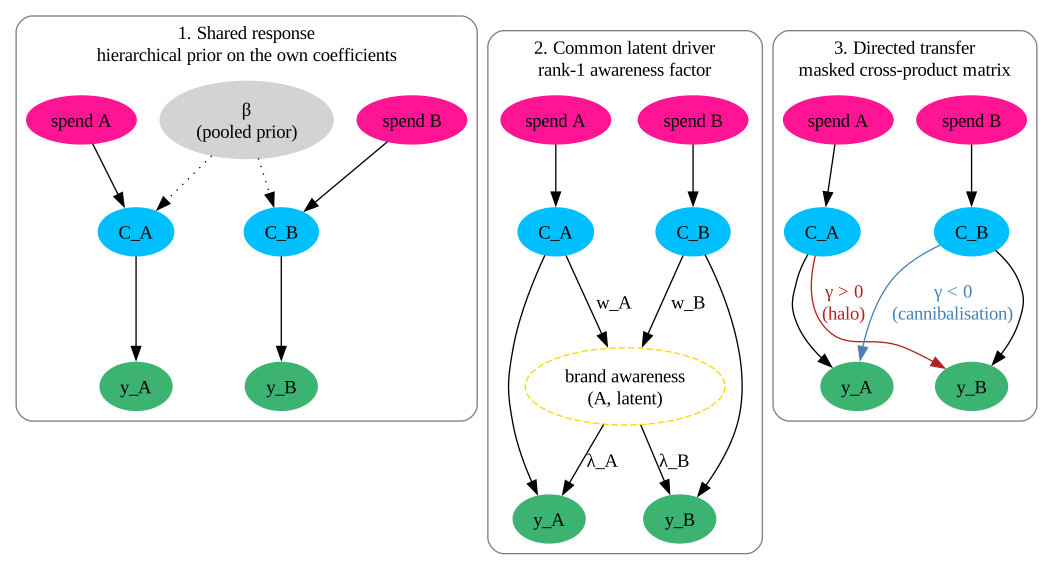
It helps to name the mechanism before choosing a parameterisation, because different mechanisms imply different structures and different failure modes. Three common ones, drawn as causal graphs below:
Shared response. Products respond similarly to the same channel. This is not a halo effect, it is a pooling question, and the right answer is a hierarchical prior over the per-product channel coefficients. If you model it as a cross-product term you will find “halo” everywhere.
A common latent driver. One unobserved quantity (brand awareness, seasonality, distribution) moves all products together, and media feeds it. A rank-1 latent factor is the natural parameterisation.
Directed product-to-product transfer. Media on \(j\) changes demand for \(i\) specifically, with a direction and a sign. This is what people usually mean by halo and cannibalisation, and it needs an explicit cross term.
Mechanisms 2 and 3 are what we model below. Mechanism 1 is a warning: check that a hierarchical baseline does not already explain the correlation before reaching for a cross-product matrix.
The graphs make the distinction sharp. Only mechanism 3 has an arrow from one product’s media into another product’s demand. Mechanism 1 has no such arrow at all: the products are linked through a shared prior on their own coefficients, which is a statement about our uncertainty rather than about the world. Mechanism 2 routes every product’s media through one shared node, so it cannot lift one sibling while hurting another.
import graphviz as gr

SPEND_STYLE = {"color": "deeppink", "style": "filled"}
CONTRIBUTION_STYLE = {"color": "deepskyblue", "style": "filled"}
TARGET_STYLE = {"color": "mediumseagreen", "style": "filled"}
LATENT_STYLE = {"color": "gold", "style": "dashed"}
PARAMETER_STYLE = {"color": "lightgray", "style": "filled"}
HALO_STYLE = {"color": "firebrick", "fontcolor": "firebrick"}
CANNIBALISATION_STYLE = {"color": "steelblue", "fontcolor": "steelblue"}

NodeSpec = dict[str, tuple[str, dict[str, str]]]
EdgeSpec = list[tuple[str, str, dict[str, str]]]

# Two products with their own-media paths. Every mechanism adds to this skeleton.
BASE_NODES: NodeSpec = {
    "xa": ("spend A", SPEND_STYLE),
    "xb": ("spend B", SPEND_STYLE),
    "Ca": ("C_A", CONTRIBUTION_STYLE),
    "Cb": ("C_B", CONTRIBUTION_STYLE),
    "ya": ("y_A", TARGET_STYLE),
    "yb": ("y_B", TARGET_STYLE),
}
BASE_EDGES: EdgeSpec = [
    ("xa", "Ca", {}),
    ("xb", "Cb", {}),
    ("Ca", "ya", {}),
    ("Cb", "yb", {}),
]


def add_mechanism(
    graph: gr.Digraph, name: str, label: str, nodes: NodeSpec, edges: EdgeSpec
) -> None:
    """Draw one mechanism as a labelled cluster inside ``graph``."""
    with graph.subgraph(name=f"cluster_{name}") as cluster:
        cluster.attr(label=label, labelloc="t", style="rounded", color="gray50")
        for node, (node_label, attrs) in nodes.items():
            cluster.node(f"{name}_{node}", node_label, **attrs)
        for parent, child, attrs in edges:
            cluster.edge(f"{name}_{parent}", f"{name}_{child}", **attrs)


mechanisms = gr.Digraph()
mechanisms.attr("node", shape="ellipse")

add_mechanism(
    mechanisms,
    "shared",
    "1. Shared response\nhierarchical prior on the own coefficients",
    BASE_NODES | {"beta": ("β\n(pooled prior)", PARAMETER_STYLE)},
    [
        *BASE_EDGES,
        ("beta", "Ca", {"style": "dotted"}),
        ("beta", "Cb", {"style": "dotted"}),
    ],
)
add_mechanism(
    mechanisms,
    "latent",
    "2. Common latent driver\nrank-1 awareness factor",
    BASE_NODES | {"A": ("brand awareness\n(A, latent)", LATENT_STYLE)},
    [
        *BASE_EDGES,
        ("Ca", "A", {"label": "w_A"}),
        ("Cb", "A", {"label": "w_B"}),
        ("A", "ya", {"label": "λ_A"}),
        ("A", "yb", {"label": "λ_B"}),
    ],
)
add_mechanism(
    mechanisms,
    "transfer",
    "3. Directed transfer\nmasked cross-product matrix",
    BASE_NODES,
    [
        *BASE_EDGES,
        ("Ca", "yb", {"label": "γ > 0\n(halo)", **HALO_STYLE}),
        ("Cb", "ya", {"label": "γ < 0\n(cannibalisation)", **CANNIBALISATION_STYLE}),
    ],
)

mechanisms
Tip
How to read the graphs. Filled nodes are observed or computed by the model: spend (pink), the adstocked and saturated contribution \(C\) (blue), and the target \(y\) (green). A dashed outline marks a latent quantity that no dataset contains. Dotted arrows are prior links between parameters rather than causal edges. Red arrows are halos and blue arrows cannibalisation, matching the colour scale of the estimated cross-effect matrix at the end of the notebook.
The standard multi-dimensional MMM#
The MMM class with dims=("product",) estimates
where \(f_m\) chains adstock with saturation. We write \(C_{t,i}\) for product \(i\)’s total media contribution at time \(t\). The key structural fact is that \(C_{t,i}\) depends only on product \(i\)’s own spend. There is no coupling.
Where the cross term belongs#
The design question is what signal the cross term reads, and this is the single most consequential choice in the notebook.
Read the transformed contribution, not raw spend. The cross term should read \(C_{t,j}\), the already-adstocked and already-saturated contribution of the source product, and apply a plain linear coefficient to it:
Transform once, read linearly many times. The carryover and diminishing-returns structure is estimated once per source product from that product’s own response, and every downstream reader inherits it. No new adstock or saturation parameters have to be estimated for the cross term.
This is a short parametrization, not a structurally different model. Write the fully general alternative as a second, independent pathway from the source’s spend into the receiver, with its own adstock and its own saturation per channel. Because the amplitude \(\beta_{m,j}\) enters \(C_{t,j} = \sum_m \beta_{m,j} f_m(\cdot)\) linearly, the cross term is exactly that general model with the adstock and saturation shape parameters completely pooled with the source’s own pathway, and only the amplitude left free:
The cross pathway therefore still carries a full adstock and a full saturation per channel, the same curves as the own pathway rescaled, and the only new parameter per pair is the effective amplitude \(\gamma_{ij}\beta_{m,j}\). What the pooling assumes is that spillover inherits the source’s carryover and curvature; if a pair genuinely needs its own shape, that is the point at which to write the second transformation out explicitly, keeping a saturation on it for the reason below.
The alternative, giving the cross term its own transformation of the source’s raw spend, has a specific failure mode worth naming. A cross term on raw spend without saturation grows without bound while the own-effect saturates, so at high spend the model can always improve the fit by shovelling more lift into the halo term. The fitted halo then keeps rising exactly where the direct effect flattens, and a budget optimiser reading that model will push spend to the top of the range. If you do want a raw-spend cross term, keep a saturation on it.
Sign-free by default. \(\gamma_{ij}\) carries a Normal prior centred at
zero, not a HalfNormal. A positive-only prior cannot express
cannibalisation, and worse, it does not fail loudly: the posterior simply
piles up near zero and the model reports “no effect” for a product that is
in fact being cannibalised. We demonstrate this failure explicitly below.
One coefficient is a net, not a decomposition. \(\gamma_{ij}\) is the net of every halo and every cannibalisation channel running from \(j\) to \(i\). A pair that has both a real awareness halo and a real substitution loss will report their difference. Splitting them requires channel-resolved sources (a brand-building channel and a promotional channel entering separately), not a finer prior.
The diagonal is always masked out. \(\gamma_{ii}\) and the own-effect \(C_{t,i}\) read the same signal, so leaving both free makes them unidentifiable up to a shift. Own effects go through \(C_{t,i}\); cross effects go through \(\gamma\); never both.
The mask is the model#
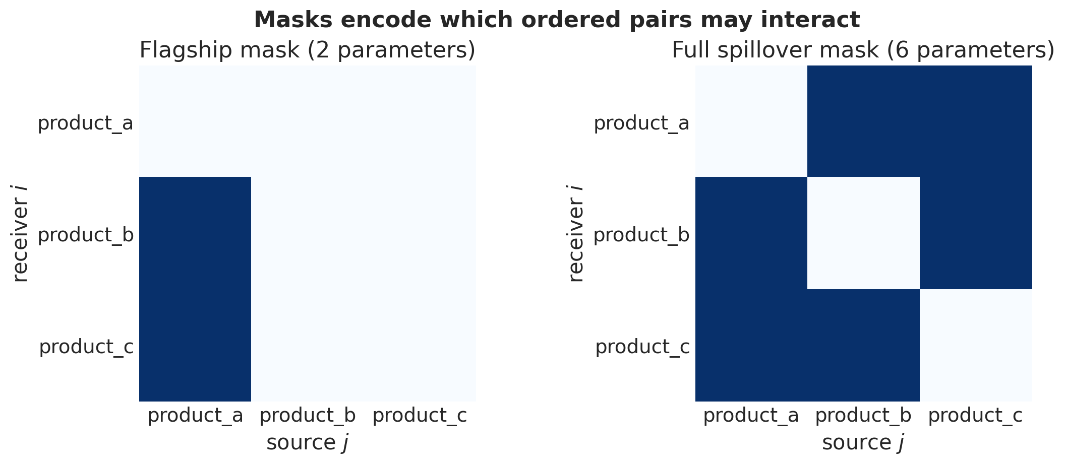
With \(P\) products, a free matrix has \(P(P-1)\) off-diagonal parameters. At
\(P=3\) that is 6, at \(P=12\) it is 132, and the data rarely support them. Rather
than write a different class per structure, we write one effect that takes
a boolean mask over ordered pairs (product, product_source) and estimates a
coefficient only where the mask is True. Many of the structures in the
literature are then a choice of mask:
Mask |
Active entries |
Parameters |
Assumption |
|---|---|---|---|
Flagship |
one source column |
\(P-1\) |
a single known awareness driver |
Full spillover |
all off-diagonal |
\(P(P-1)\) |
any product may affect any other |
Block / family |
within-family blocks |
\(\sum_f P_f(P_f-1)\) |
transfer happens inside a family |
Hierarchy |
upper-triangular |
\(P(P-1)/2\) |
premium lifts standard, not the reverse |
The mask is where business knowledge enters the model, and it is a stronger and more honest lever than a tighter prior: it says this pair cannot interact, which is usually a claim the business can actually defend, whereas this coefficient is small usually is not.
Masking alone is not enough at scale. We pair it with a global shrinkage hyperprior on the coefficient scale, so the active entries are pulled to zero unless the data argue otherwise.
We also fit two contrasts: the latent brand-awareness factor (mechanism 2, a rank-1 approximation \(\gamma_{ij} \approx \lambda_i w_j\) with \(2P\) sampled parameters), and the simplest available workaround, other products’ total spend as an extra channel, which needs no new machinery at all but cannot say which product the spillover came from.
Simulation design#
We generate synthetic data from a known cross-product structure and check what each approach recovers.
Crucially, the ground truth contains one positive and one negative cross effect. Product B enjoys a halo from the flagship; product C is cannibalised by it. A notebook whose ground truth is all-positive cannot detect the sign-restriction failure that motivates most of the design above.
Generate spend, set ground-truth parameters by hand, forward-sample with
pymc.do()+sample_prior_predictive().Fit a baseline MMM with no cross term.
Fit the aggregate-other-spend workaround.
Fit the masked cross-product effect under the flagship mask and the full spillover mask.
Refit the flagship mask with a
HalfNormalcoefficient to show what a sign restriction costs.Fit the latent brand-awareness factor.
Compare recovery, portfolio-level contribution bias, and identifiability.
Prepare notebook#
import arviz as az
import arviz_plots as azp
import matplotlib.pyplot as plt
import numpy as np
import pandas as pd
import pymc as pm
import pymc.dims as pmd
import xarray as xr
from matplotlib.axes import Axes
from matplotlib.figure import Figure
from pydantic import InstanceOf
from pymc import do
from pymc_extras.prior import Prior
from pytensor.xtensor.type import XTensorVariable

from pymc_marketing.metrics import crps
from pymc_marketing.mmm import GeometricAdstock, LogisticSaturation
from pymc_marketing.mmm.additive_effect import MuEffect
from pymc_marketing.mmm.mmm import MMM
from pymc_marketing.mmm.transformers import geometric_adstock, logistic_saturation
from pymc_marketing.special_priors import MaskedPrior

az.style.use("arviz-darkgrid")
plt.rcParams["figure.figsize"] = [10, 6]
plt.rcParams["figure.dpi"] = 100
plt.rcParams["figure.facecolor"] = "white"

%config InlineBackend.figure_format = "retina"
/Users/juanitorduz/Documents/pymc-marketing/.venv/lib/python3.14/site-packages/tqdm/auto.py:21: TqdmWarning: IProgress not found. Please update jupyter and ipywidgets. See https://ipywidgets.readthedocs.io/en/stable/user_install.html
  from .autonotebook import tqdm as notebook_tqdm
seed: int = sum(map(ord, "halo"))
rng: np.random.Generator = np.random.default_rng(seed=seed)
Simulation parameters#
PRODUCTS: list[str] = ["product_a", "product_b", "product_c"]
CHANNELS: list[str] = ["tv", "digital"]
FLAGSHIP: str = "product_a"
FLAGSHIP_IDX: int = PRODUCTS.index(FLAGSHIP)
RECEIVERS: list[str] = [product for product in PRODUCTS if product != FLAGSHIP]

N_DATES: int = 110
L_MAX: int = 8
DATE_RANGE = pd.date_range(start="2022-01-03", freq="W-MON", periods=N_DATES)

SAMPLER_CONFIG: dict = {
    "nuts_sampler": "nutpie",
    "chains": 4,
    "draws": 1_000,
    "tune": 1_000,
    "random_seed": rng,
}

N_PRODUCTS = len(PRODUCTS)
N_CHANNELS = len(CHANNELS)
Synthetic data generation#
We follow the do() + sample_prior_predictive() pattern from
Generating Synthetic MMM Data.
Generate channel spend#
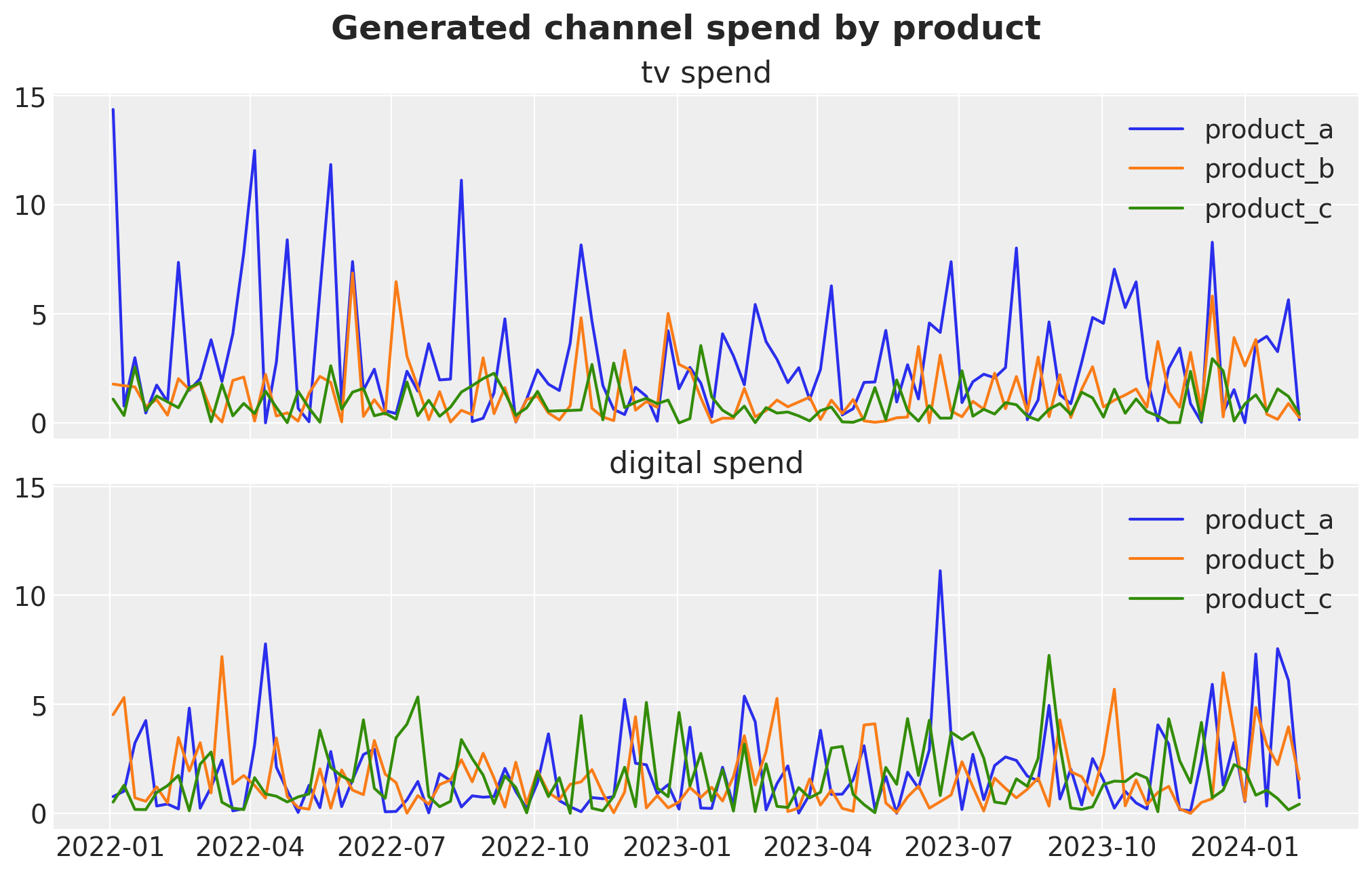
First, we generate the spend data.
spend_scales = {
    "product_a": {"tv": 3.0, "digital": 2.0},
    "product_b": {"tv": 1.5, "digital": 1.8},
    "product_c": {"tv": 1.0, "digital": 1.5},
}

spend_df = pd.concat(
    [
        pd.DataFrame(
            {
                "date": DATE_RANGE,
                "product": product,
                **{
                    channel: pm.draw(
                        pm.Exponential.dist(lam=1 / spend_scales[product][channel]),
                        draws=N_DATES,
                        random_seed=rng,
                    )
                    for channel in CHANNELS
                },
            }
        )
        for product in PRODUCTS
    ],
    ignore_index=True,
)
spend_df.head()
| date | product | tv | digital | |
|---|---|---|---|---|
| 0 | 2022-01-03 | product_a | 14.377020 | 0.778108 |
| 1 | 2022-01-10 | product_a | 0.778700 | 1.025356 |
| 2 | 2022-01-17 | product_a | 2.996377 | 3.230748 |
| 3 | 2022-01-24 | product_a | 0.459857 | 4.263118 |
| 4 | 2022-01-31 | product_a | 1.740401 | 0.345552 |
Let’s visualise it:
fig, axes = plt.subplots(
    nrows=N_CHANNELS, ncols=1, sharex=True, sharey=True, layout="constrained"
)
for ax, channel in zip(axes, CHANNELS, strict=True):
    for product in PRODUCTS:
        _prod_df = spend_df.query("product == @product")
        ax.plot(_prod_df["date"], _prod_df[channel], label=product)
    ax.set_title(f"{channel} spend")
    ax.legend()
fig.suptitle(
    "Generated channel spend by product", fontsize=18, fontweight="bold", y=1.05
);
Set ground-truth parameters#
The truths are set by hand rather than drawn from the priors, and the choice is not cosmetic. The cross coefficient is identified by the temporal variation of the flagship’s transformed contribution \(C_{t,\text{flagship}}\): the receiver’s intercept absorbs any constant level, so only the movement of \(C_{t,\text{flagship}}\) carries information about \(\gamma\). If a flagship channel sits deep in saturation, its contribution flattens into a near constant, and the halo becomes unidentifiable no matter how large it is. We therefore place every channel in a mid-saturation regime, \(\lambda \cdot \bar{x} \approx 1\) on the adstocked spend, which keeps the saturation curve responsive and gives \(C_{t,\text{flagship}}\) enough temporal variation to read a coefficient off. Both quantities are computed on the generated data below rather than asserted. This is worth checking in real data too: a halo read off an always-on, fully saturated flagship is a claim the data cannot support.
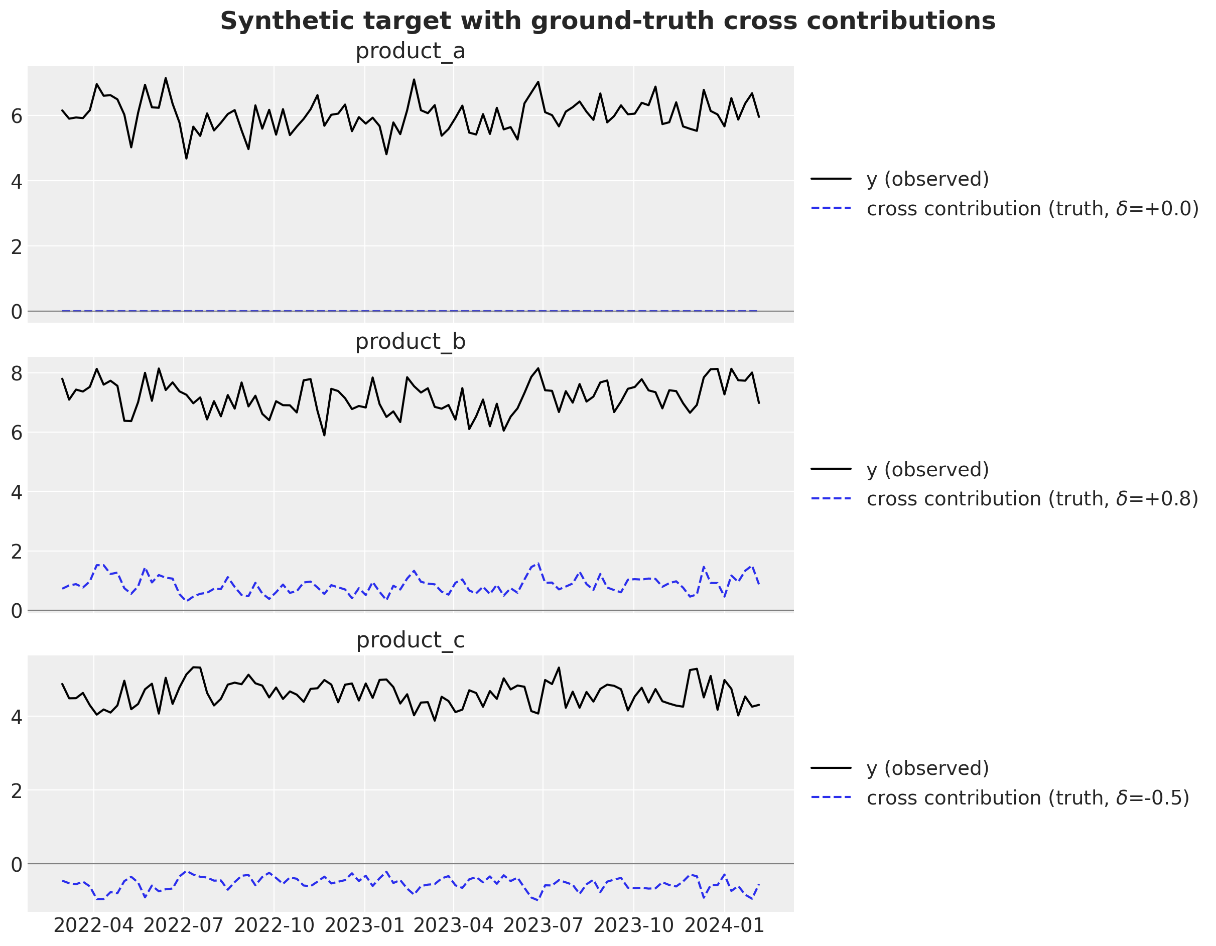
The halo vector is the important line. product_a is the flagship and has no
self-halo. product_b receives a positive halo of 0.8. product_c is
cannibalised at -0.5: every unit of flagship contribution costs it
0.5 units of demand.
intercept_true = np.array([5.0, 5.5, 4.5])

adstock_alpha_true = np.array([[0.5, 0.3], [0.4, 0.2], [0.3, 0.4]])
saturation_lam_true = np.array([[0.35, 0.5], [0.7, 0.6], [1.0, 0.7]])
saturation_beta_true = np.array([[1.5, 1.0], [1.2, 0.9], [0.8, 0.7]])

# No self-halo, positive halo on product_b, cannibalisation on product_c.
delta_true = np.array([0.0, 0.8, -0.5])

sigma_true = np.array([0.25, 0.25, 0.25])

pd.DataFrame(
    {
        "adstock alpha": adstock_alpha_true.ravel(),
        "saturation lam": saturation_lam_true.ravel(),
        "saturation beta": saturation_beta_true.ravel(),
    },
    index=pd.MultiIndex.from_product(
        [PRODUCTS, CHANNELS], names=["product", "channel"]
    ),
).join(
    pd.DataFrame(
        {
            "intercept": intercept_true,
            "halo delta": delta_true,
            "sigma": sigma_true,
        },
        index=pd.Index(PRODUCTS, name="product"),
    ),
    on="product",
)
| adstock alpha | saturation lam | saturation beta | intercept | halo delta | sigma | ||
|---|---|---|---|---|---|---|---|
| product | channel | ||||||
| product_a | tv | 0.5 | 0.35 | 1.5 | 5.0 | 0.0 | 0.25 |
| digital | 0.3 | 0.50 | 1.0 | 5.0 | 0.0 | 0.25 | |
| product_b | tv | 0.4 | 0.70 | 1.2 | 5.5 | 0.8 | 0.25 |
| digital | 0.2 | 0.60 | 0.9 | 5.5 | 0.8 | 0.25 | |
| product_c | tv | 0.3 | 1.00 | 0.8 | 4.5 | -0.5 | 0.25 |
| digital | 0.4 | 0.70 | 0.7 | 4.5 | -0.5 | 0.25 |
Build the DGP and forward-sample#
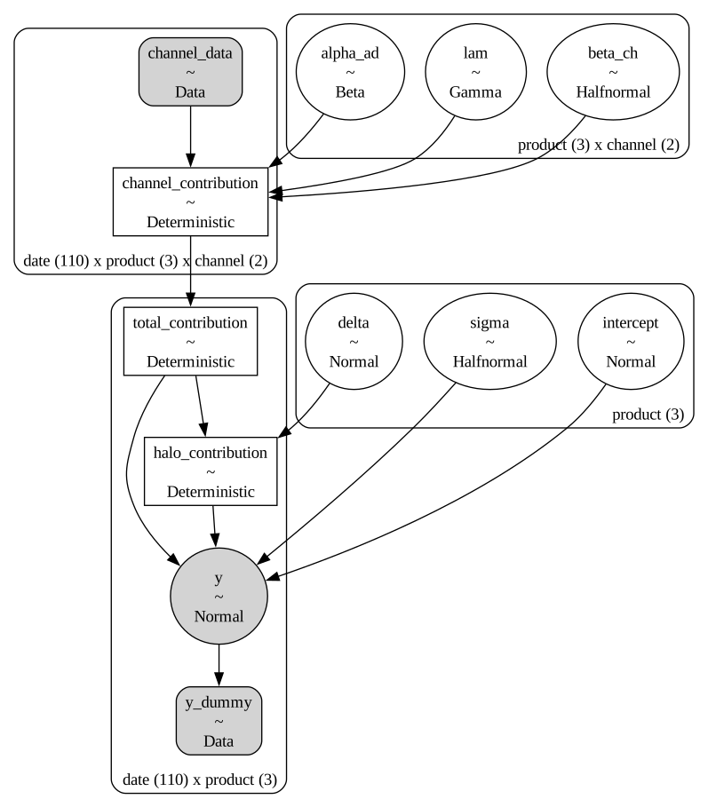
The cross term reads total_contribution for the flagship, which is already
adstocked and saturated, and multiplies it by a plain coefficient. The
coefficient is drawn from a Normal, so the DGP is sign-free in exactly the
way the models below need to be.
channel_spend_3d = np.zeros((N_DATES, N_PRODUCTS, N_CHANNELS))
for ip, product in enumerate(PRODUCTS):
    mask_p = spend_df["product"] == product
    for ic, channel in enumerate(CHANNELS):
        channel_spend_3d[:, ip, ic] = spend_df.loc[mask_p, channel].values

dgp_coords = {"date": DATE_RANGE, "product": PRODUCTS, "channel": CHANNELS}

with pm.Model(coords=dgp_coords) as dgp_model:
    channel_data = pmd.Data(
        "channel_data", channel_spend_3d, dims=("date", "product", "channel")
    )
    y_dummy = pmd.Data(
        "y_dummy", np.ones((N_DATES, N_PRODUCTS)), dims=("date", "product")
    )

    alpha_ad = pmd.Beta("alpha_ad", alpha=1, beta=3, dims=("product", "channel"))
    adstocked = geometric_adstock(
        channel_data, alpha=alpha_ad, l_max=L_MAX, dim="date", normalize=True
    )

    lam = pmd.Gamma("lam", alpha=2, beta=1, dims=("product", "channel"))
    beta_ch = pmd.HalfNormal("beta_ch", sigma=1, dims=("product", "channel"))
    channel_contribution = pmd.Deterministic(
        "channel_contribution",
        (beta_ch * logistic_saturation(adstocked, lam)).transpose("date", ...),
    )

    total = pmd.Deterministic(
        "total_contribution", channel_contribution.sum(dim="channel")
    )
    flagship_total = total.isel(product=FLAGSHIP_IDX)

    # Sign-free: the DGP can produce cannibalisation as well as halo.
    delta = pmd.Normal("delta", mu=0, sigma=1, dims="product")
    halo_contribution = pmd.Deterministic(
        "halo_contribution", (delta * flagship_total).transpose("date", ...)
    )

    intercept = pmd.Normal("intercept", mu=5, sigma=1, dims="product")
    mu = (intercept + total + halo_contribution).transpose("date", "product")

    sigma = pmd.HalfNormal("sigma", sigma=0.5, dims="product")
    pmd.Normal("y", mu=mu, sigma=sigma, observed=y_dummy, dims=("date", "product"))

pm.model_to_graphviz(dgp_model)
dgp_model_do = do(
    dgp_model,
    {
        "intercept": intercept_true,
        "alpha_ad": adstock_alpha_true,
        "lam": saturation_lam_true,
        "beta_ch": saturation_beta_true,
        "delta": delta_true,
        "sigma": sigma_true,
    },
)

with dgp_model_do:
    idata_dgp = pm.sample_prior_predictive(draws=1, random_seed=rng)
Sampling: [y]
y_obs = idata_dgp["prior_predictive"]["y"].sel(chain=0, draw=0).values

channel_contribution_true_xr = idata_dgp["prior"]["channel_contribution"].sel(
    chain=0, draw=0
)
halo_contribution_true_xr = idata_dgp["prior"]["halo_contribution"].sel(chain=0, draw=0)
total_contribution_true_xr = idata_dgp["prior"]["total_contribution"].sel(
    chain=0, draw=0
)

# Trim the adstock burn-in.
trim = L_MAX
date_range_trimmed = DATE_RANGE[trim:]
y_obs_trimmed = y_obs[trim:]
channel_contribution_true_trimmed = channel_contribution_true_xr.values[trim:]
channel_spend_trimmed = channel_spend_3d[trim:]
halo_contribution_true_trimmed = halo_contribution_true_xr.values[trim:]
total_contribution_true_trimmed = total_contribution_true_xr.values[trim:]

n_dates_trimmed = len(date_range_trimmed)

rows_final = []
for ip, product in enumerate(PRODUCTS):
    for it, date in enumerate(date_range_trimmed):
        row = {"date": date, "product": product}
        for ic, channel in enumerate(CHANNELS):
            row[channel] = channel_spend_trimmed[it, ip, ic]
        row["y"] = y_obs_trimmed[it, ip]
        rows_final.append(row)

data_df = pd.DataFrame(rows_final)
data_df.head()
| date | product | tv | digital | y | |
|---|---|---|---|---|---|
| 0 | 2022-02-28 | product_a | 2.037748 | 0.244770 | 6.158224 |
| 1 | 2022-03-07 | product_a | 3.817663 | 1.212383 | 5.904474 |
| 2 | 2022-03-14 | product_a | 1.903096 | 2.445819 | 5.941831 |
| 3 | 2022-03-21 | product_a | 4.091189 | 0.123654 | 5.922206 |
| 4 | 2022-03-28 | product_a | 7.784267 | 0.222690 | 6.164689 |
Both claims made when the truths were set are checked here rather than asserted: every channel sits near \(\lambda \bar{x} \approx 1\) on the adstocked spend, and each product’s total contribution has a coefficient of variation of \(0.3\)–\(0.4\), so there is movement for a cross coefficient to read.
adstocked_true = xr.DataArray(
    pm.draw(
        geometric_adstock(
            xr.DataArray(
                channel_spend_3d,
                dims=("date", "product", "channel"),
                coords={"date": DATE_RANGE, "product": PRODUCTS, "channel": CHANNELS},
            ),
            alpha=xr.DataArray(
                adstock_alpha_true,
                dims=("product", "channel"),
                coords={"product": PRODUCTS, "channel": CHANNELS},
            ),
            l_max=L_MAX,
            dim="date",
            normalize=True,
        )
    ),
    dims=("product", "channel", "date"),
    coords={"product": PRODUCTS, "channel": CHANNELS, "date": DATE_RANGE},
).isel(date=slice(trim, None))

identification_df = pd.DataFrame(
    saturation_lam_true * adstocked_true.mean("date").values,
    index=PRODUCTS,
    columns=[f"lam*xbar {channel}" for channel in CHANNELS],
).assign(
    **{
        "contribution CV": total_contribution_true_trimmed.std(axis=0)
        / total_contribution_true_trimmed.mean(axis=0)
    }
)
identification_df.index.name = "product"
identification_df.round(2)
| lam*xbar tv | lam*xbar digital | contribution CV | |
|---|---|---|---|
| product | |||
| product_a | 1.04 | 0.92 | 0.34 |
| product_b | 0.95 | 0.94 | 0.38 |
| product_c | 0.88 | 1.20 | 0.33 |
The ground-truth cross contribution is positive for product_b and negative
for product_c, tracking the flagship’s media in both cases.
fig, axes = plt.subplots(
    nrows=N_PRODUCTS,
    ncols=1,
    figsize=(12, 3 * N_PRODUCTS),
    sharex=True,
    layout="constrained",
)
for ip, product in enumerate(PRODUCTS):
    ax = axes[ip]
    _prod_df = data_df.query("product == @product")
    ax.plot(_prod_df["date"], _prod_df["y"], c="black", label="y (observed)")
    ax.plot(
        date_range_trimmed,
        halo_contribution_true_trimmed[:, ip],
        label=f"cross contribution (truth, $\\delta$={delta_true[ip]:+.1f})",
        c="C0",
        linestyle="--",
    )
    ax.axhline(0, c="gray", lw=0.8)
    ax.legend(loc="center left", bbox_to_anchor=(1, 0.5))
    ax.set_title(product)
fig.suptitle(
    "Synthetic target with ground-truth cross contributions",
    fontsize=18,
    fontweight="bold",
    y=1.03,
);
Baseline: standard MMM, no cross term#
This model has no mechanism for cross-product transfer, so the halo and the cannibalisation have to be absorbed by the intercept and the own-channel coefficients.
X = data_df[["date", "product", *CHANNELS]]
y = data_df["y"]

mmm_baseline = MMM(
    date_column="date",
    channel_columns=CHANNELS,
    target_column="y",
    adstock=GeometricAdstock(l_max=L_MAX),
    saturation=LogisticSaturation(),
    dims=("product",),
)
mmm_baseline.build_model(X, y)
mmm_baseline.add_original_scale_contribution_variable(var=["channel_contribution", "y"])
mmm_baseline.fit(X=X, y=y, **SAMPLER_CONFIG)
mmm_baseline.sample_posterior_predictive(X=X, random_seed=rng);
NUTS[nutpie]: [y_sigma, adstock_alpha, saturation_lam, saturation_beta, intercept_contribution]
/Users/juanitorduz/Documents/pymc-marketing/.venv/lib/python3.14/site-packages/rich/live.py:260: UserWarning:
install "ipywidgets" for Jupyter support
  warnings.warn('install "ipywidgets" for Jupyter support')
/Users/juanitorduz/Documents/pymc-marketing/.venv/lib/python3.14/site-packages/rich/live.py:260: UserWarning:
install "ipywidgets" for Jupyter support
  warnings.warn('install "ipywidgets" for Jupyter support')
Sampling: [y]
/Users/juanitorduz/Documents/pymc-marketing/.venv/lib/python3.14/site-packages/rich/live.py:260: UserWarning:
install "ipywidgets" for Jupyter support
  warnings.warn('install "ipywidgets" for Jupyter support')
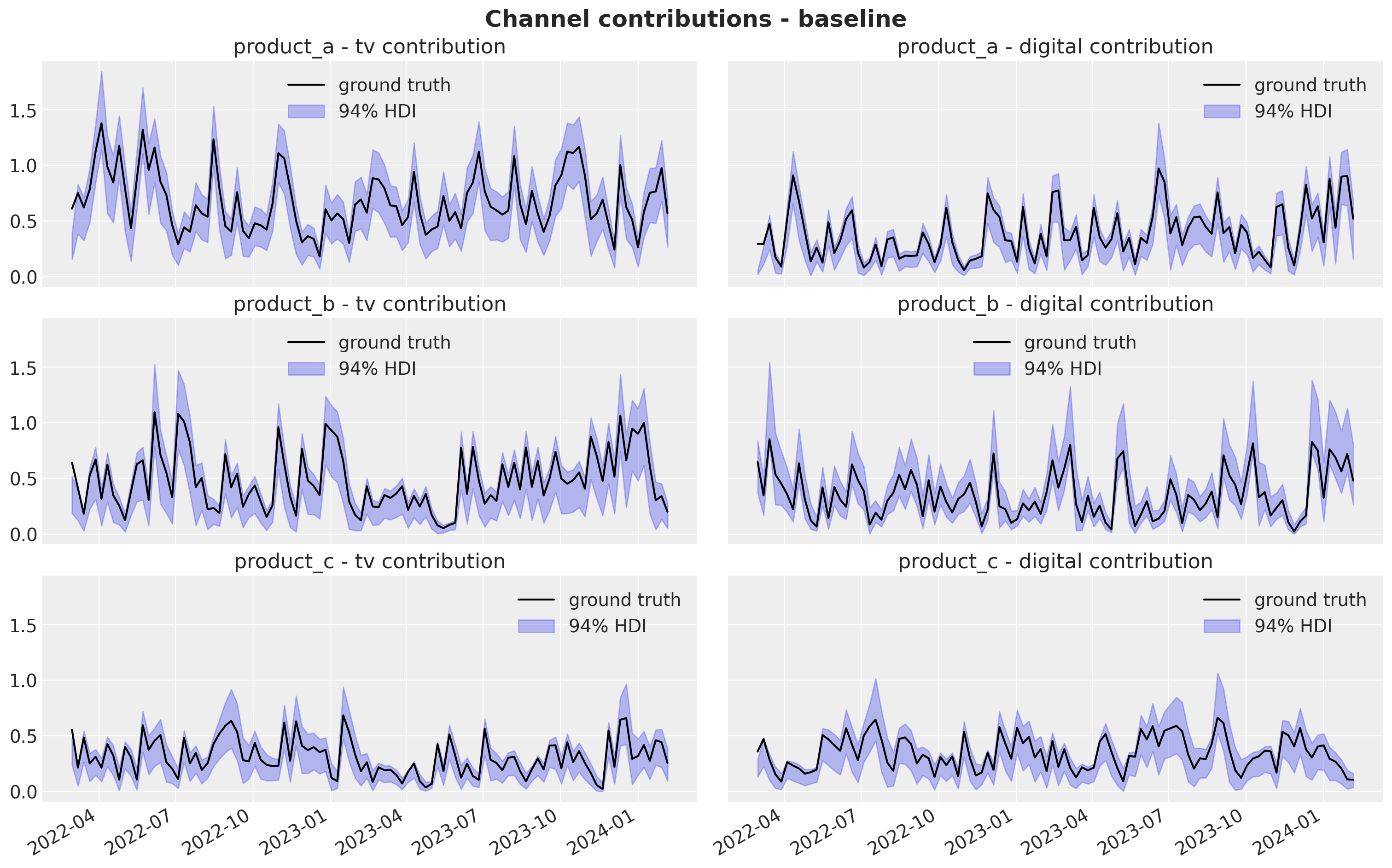
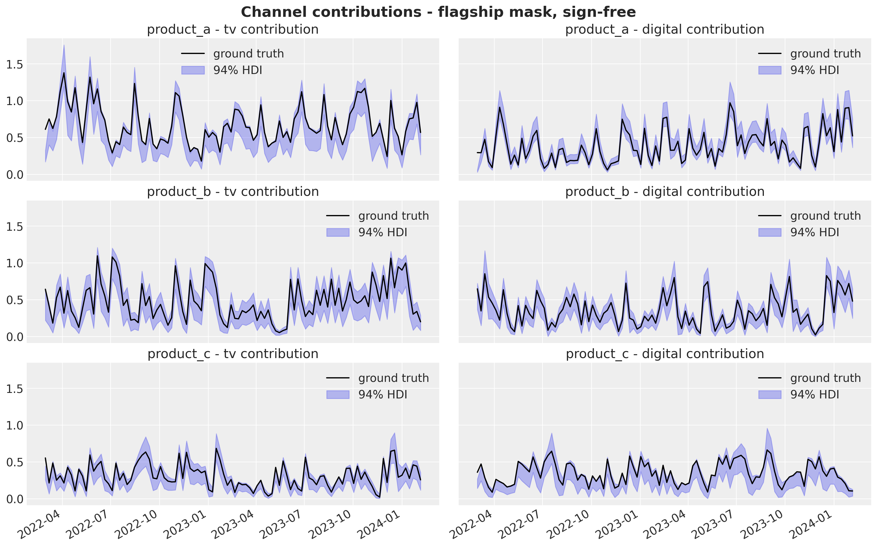
One caveat on the overlay plots that follow: the fitted models only see the
trimmed data, so their adstock warms up from zero while the ground truth
carries the full pre-trim history. The first few fitted dates are therefore
not exactly comparable; the discrepancy decays within l_max periods.
def plot_true_channel_contributions() -> tuple[Figure, np.ndarray]:
    """Grid of ground-truth channel contributions, ready to overlay estimates on."""
    fig, axes = plt.subplots(
        nrows=N_PRODUCTS,
        ncols=N_CHANNELS,
        figsize=(15, 3 * N_PRODUCTS),
        sharex=True,
        sharey=True,
        layout="constrained",
    )
    for ip, product in enumerate(PRODUCTS):
        for ic, channel in enumerate(CHANNELS):
            ax = axes[ip, ic]
            ax.plot(
                date_range_trimmed,
                channel_contribution_true_trimmed[:, ip, ic],
                c="black",
                label="ground truth",
            )
            ax.legend()
            ax.set_title(f"{product} - {channel} contribution")
    fig.autofmt_xdate()
    return fig, axes


def hdi_bounds(
    da: xr.DataArray, prob: float = 0.94
) -> tuple[xr.DataArray, xr.DataArray]:
    """Return (lower, upper) HDI DataArrays for a posterior DataArray."""
    h = az.hdi(da, prob=prob)
    if isinstance(h, xr.Dataset):
        h = h[next(iter(h.data_vars))]
    return h.sel(ci_bound="lower"), h.sel(ci_bound="upper")


def bare(da: xr.DataArray) -> xr.DataArray:
    """Drop chain/draw coordinate labels so arrays combine positionally."""
    return da.drop_vars([c for c in ("chain", "draw") if c in da.coords])


def overlay_channel_contributions(
    mmm_obj: MMM, title: str
) -> tuple[Figure, np.ndarray]:
    """Overlay a fitted model's channel-contribution HDI on the ground truth."""
    fig, axes = plot_true_channel_contributions()
    post = mmm_obj.idata["posterior"]["channel_contribution_original_scale"]
    for ip, product in enumerate(PRODUCTS):
        for ic, channel in enumerate(CHANNELS):
            ax = axes[ip, ic]
            lo, hi = hdi_bounds(post.sel(product=product, channel=channel))
            ax.fill_between(
                date_range_trimmed, lo, hi, color="C0", alpha=0.3, label="94% HDI"
            )
            ax.legend()
    fig.suptitle(title, fontsize=18, fontweight="bold", y=1.03)
    return fig, axes


overlay_channel_contributions(mmm_baseline, "Channel contributions - baseline");
Workaround: other products’ total spend as a channel#
The cheapest thing that can possibly work. For each product, sum the raw media
spend of every other product and pass it as an extra channel column. The
MMM class then gives it its own adstock and saturation.
This costs no new machinery and it does saturate the cross signal, which
avoids the unbounded-growth failure described earlier. What it cannot do is
say which product the spillover came from, or carry a sign per source, so it
collapses a halo from one sibling and a cannibalisation from another into a
single coefficient. And because the default saturation coefficient prior is a
HalfNormal, that single coefficient is positive-only: the workaround
inherits exactly the sign-restriction failure we demonstrate below, and a
cannibalised product will read as “no spillover”.
data_df["total_spend"] = data_df[CHANNELS].sum(axis=1)
date_total_spend = data_df.groupby("date")["total_spend"].transform("sum")
data_df["other_products_total_media"] = date_total_spend - data_df["total_spend"]

X_other = data_df[["date", "product", *CHANNELS, "other_products_total_media"]]

mmm_other_spend = MMM(
    date_column="date",
    channel_columns=[*CHANNELS, "other_products_total_media"],
    target_column="y",
    adstock=GeometricAdstock(l_max=L_MAX),
    saturation=LogisticSaturation(),
    dims=("product",),
)
mmm_other_spend.build_model(X_other, y)
mmm_other_spend.add_original_scale_contribution_variable(
    var=["channel_contribution", "y"]
)
mmm_other_spend.fit(X=X_other, y=y, **SAMPLER_CONFIG)
mmm_other_spend.sample_posterior_predictive(X=X_other, random_seed=rng);
NUTS[nutpie]: [y_sigma, adstock_alpha, saturation_lam, saturation_beta, intercept_contribution]
/Users/juanitorduz/Documents/pymc-marketing/.venv/lib/python3.14/site-packages/rich/live.py:260: UserWarning:
install "ipywidgets" for Jupyter support
  warnings.warn('install "ipywidgets" for Jupyter support')
/Users/juanitorduz/Documents/pymc-marketing/.venv/lib/python3.14/site-packages/rich/live.py:260: UserWarning:
install "ipywidgets" for Jupyter support
  warnings.warn('install "ipywidgets" for Jupyter support')
Sampling: [y]
/Users/juanitorduz/Documents/pymc-marketing/.venv/lib/python3.14/site-packages/rich/live.py:260: UserWarning:
install "ipywidgets" for Jupyter support
  warnings.warn('install "ipywidgets" for Jupyter support')
A single masked cross-product effect#
The MMM class exposes an extensibility hook called MuEffect, defined in
pymc_marketing.mmm.additive_effect. Any object implementing create_data,
create_effect and set_data can be appended to mmm.mu_effects before
build_model. create_effect runs after channel_contribution has been
registered as a pmd.Deterministic, which is precisely what lets a cross term
read the already-transformed contribution.
Three implementation details are worth pointing out.
The deterministic is named
f"{prefix}_effect_contribution". That is the nameMMM.compute_counterfactual_contributions_datasetlooks for viaMuEffect.contribution_var_name. An effect that registers some other name silently drops out of the contribution decomposition.MaskedPriorcreates the coefficient over the active entries of the mask only, and expands back to the full \((P, P)\) shape with exact zeros elsewhere. Masked-out pairs cost no parameters and add no sampler geometry.The coefficient prior is
Normal(0, sigma)withsigmaitself estimated, giving global shrinkage across the active entries. Sign-free, and pulled to zero unless the data argue otherwise. The scale of the shrinkage hyperprior should match the plausible size of a cross effect: we useHalfNormal(0.5), which comfortably covers coefficients up to about one while still shrinking noise. With only a handful of active entries the hyperprior is informative, and a too-tight choice (sayHalfNormal(0.1)against a true effect of0.8) would drag every estimate toward zero. At larger \(P\) with mostly-null entries, tighten it.
class CrossProductHaloEffect(MuEffect):
    """Sign-free halo and cannibalisation on an already-transformed source signal.

    Adds ``sum_j gamma_ij * C_{t,j}`` to the mean of product ``i``, where
    ``C_{t,j}`` is product ``j``'s total channel contribution (adstocked and
    saturated) and ``gamma`` is estimated only on the active entries of ``mask``.

    Parameters
    ----------
    mask : xarray.DataArray
        Boolean array over ``(product_dim, source_dim)``. ``True`` marks an
        ordered pair whose coefficient is estimated. The diagonal should be
        ``False``: own effects belong in ``channel_contribution``.
    coefficient : Prior, optional
        Prior on ``gamma``. Defaults to ``Normal(0, HalfNormal(0.5))``, which is
        sign-free with global shrinkage at a scale matched to O(1) effects.
    """

    prefix: str = "halo"
    mask: InstanceOf[xr.DataArray]
    coefficient: InstanceOf[Prior] | None = None
    product_dim: str = "product"
    source_dim: str = "product_source"

    def create_data(self, mmm: MMM) -> None:
        """Register the source coordinate mirroring the product coordinate."""
        mmm.model.add_coord(self.source_dim, list(mmm.model.coords[self.product_dim]))

    def create_effect(self, mmm: MMM) -> XTensorVariable:
        """Read the transformed contribution and apply a linear cross coefficient."""
        total = mmm.model["channel_contribution"].sum(dim="channel")
        source = total.rename({self.product_dim: self.source_dim})

        prior = self.coefficient or Prior(
            "Normal",
            mu=0,
            sigma=Prior("HalfNormal", sigma=0.5),
            dims=(self.product_dim, self.source_dim),
        )
        gamma = MaskedPrior(prior, self.mask).create_variable(
            f"{self.prefix}_gamma", xdist=True
        )
        return pmd.Deterministic(
            f"{self.prefix}_effect_contribution",
            (gamma * source).sum(dim=self.source_dim).transpose("date", ...),
        )

    def set_data(self, mmm: MMM, model: pm.Model, X: xr.Dataset) -> None:
        """No-op: the effect recomputes itself from the updated channel data."""

    def to_dict(self) -> dict:
        """Serialize, encoding the mask as plain lists."""
        return {
            "prefix": self.prefix,
            "product_dim": self.product_dim,
            "source_dim": self.source_dim,
            "coefficient": self.coefficient.to_dict() if self.coefficient else None,
            "mask": {
                "dims": list(self.mask.dims),
                "coords": {k: list(v.values) for k, v in self.mask.coords.items()},
                "values": self.mask.values.tolist(),
            },
        }

    @classmethod
    def from_dict(cls, data: dict) -> "CrossProductHaloEffect":
        """Reconstruct, rebuilding the mask DataArray."""
        work = {k: v for k, v in data.items() if k != "__type__"}
        m = work["mask"]
        coefficient = work.get("coefficient")
        return cls(
            prefix=work["prefix"],
            product_dim=work["product_dim"],
            source_dim=work["source_dim"],
            coefficient=Prior.from_dict(coefficient) if coefficient else None,
            mask=xr.DataArray(
                np.asarray(m["values"], dtype=bool), dims=m["dims"], coords=m["coords"]
            ),
        )
Building masks#
Two helpers cover the structures we fit. Both force the diagonal to False.
def make_mask(active: np.ndarray) -> xr.DataArray:
    """Wrap a boolean matrix as a (product, product_source) mask, diagonal off."""
    active = np.asarray(active, dtype=bool).copy()
    np.fill_diagonal(active, False)
    return xr.DataArray(
        active,
        dims=["product", "product_source"],
        coords={"product": PRODUCTS, "product_source": PRODUCTS},
    )


def flagship_mask(flagship: str = FLAGSHIP) -> xr.DataArray:
    """Only the flagship's column is active: one known awareness driver."""
    active = np.zeros((N_PRODUCTS, N_PRODUCTS), dtype=bool)
    active[:, PRODUCTS.index(flagship)] = True
    return make_mask(active)


def full_mask() -> xr.DataArray:
    """Every ordered off-diagonal pair is active."""
    return make_mask(np.ones((N_PRODUCTS, N_PRODUCTS), dtype=bool))


mask_flagship = flagship_mask()
mask_full = full_mask()

pd.DataFrame(
    {
        "flagship mask (active pairs)": [int(mask_flagship.values.sum())],
        "full mask (active pairs)": [int(mask_full.values.sum())],
    },
    index=["parameters"],
)
| flagship mask (active pairs) | full mask (active pairs) | |
|---|---|---|
| parameters | 2 | 6 |
fig, axes = plt.subplots(ncols=2, figsize=(11, 4.5), layout="constrained")
for ax, (m, name) in zip(
    axes,
    [(mask_flagship, "Flagship mask"), (mask_full, "Full spillover mask")],
    strict=True,
):
    ax.imshow(m.values, cmap="Blues", vmin=0, vmax=1)
    ax.grid(False)
    ax.set(
        xticks=range(N_PRODUCTS),
        yticks=range(N_PRODUCTS),
        xticklabels=PRODUCTS,
        yticklabels=PRODUCTS,
        xlabel="source $j$",
        ylabel="receiver $i$",
    )
    ax.set_title(f"{name} ({int(m.values.sum())} parameters)")
fig.suptitle(
    "Masks encode which ordered pairs may interact", fontsize=16, fontweight="bold"
);
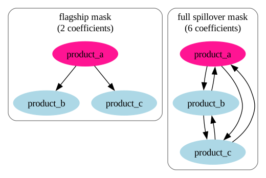
The same two masks read as causal graphs. Each arrow is one estimated coefficient, pointing from the source product’s contribution into the receiver’s demand, and the mask is precisely the claim about which arrows exist. The flagship mask asserts a single driver and no reverse paths; the full mask asserts nothing and pays for six arrows, including the reverse directions we do not expect to find.
def mask_to_dag(masks: dict[str, xr.DataArray]) -> gr.Digraph:
    """Draw each mask's active pairs as arrows from source to receiver."""
    graph = gr.Digraph()
    graph.attr("node", shape="ellipse", style="filled", color="lightblue")
    for name, mask in masks.items():
        n_active = int(mask.values.sum())
        with graph.subgraph(name=f"cluster_{name}") as cluster:
            cluster.attr(
                label=f"{name}\n({n_active} coefficients)",
                labelloc="t",
                style="rounded",
                color="gray50",
            )
            for product in PRODUCTS:
                is_flagship = product == FLAGSHIP
                cluster.node(
                    f"{name}_{product}",
                    product,
                    color="deeppink" if is_flagship else "lightblue",
                )
            for receiver in PRODUCTS:
                for source in PRODUCTS:
                    if bool(mask.sel(product=receiver, product_source=source)):
                        cluster.edge(f"{name}_{source}", f"{name}_{receiver}")
    return graph


mask_to_dag({"flagship mask": mask_flagship, "full spillover mask": mask_full})
Fitting helper#
def fit_halo_mmm(
    mask: xr.DataArray, coefficient: Prior | None = None, prefix: str = "halo"
) -> MMM:
    """Build and fit an MMM carrying a masked cross-product effect."""
    mmm_obj = MMM(
        date_column="date",
        channel_columns=CHANNELS,
        target_column="y",
        adstock=GeometricAdstock(l_max=L_MAX),
        saturation=LogisticSaturation(),
        dims=("product",),
    )
    mmm_obj.mu_effects.append(
        CrossProductHaloEffect(mask=mask, coefficient=coefficient, prefix=prefix)
    )
    mmm_obj.build_model(X, y)
    mmm_obj.add_original_scale_contribution_variable(
        var=["channel_contribution", f"{prefix}_effect_contribution", "y"]
    )
    mmm_obj.fit(X=X, y=y, **SAMPLER_CONFIG)
    mmm_obj.sample_posterior_predictive(X=X, random_seed=rng)
    return mmm_obj
Flagship mask, sign-free coefficient#
This matches the DGP: one source column, coefficients free to take either sign. It is the model we expect to recover \(\delta = [0, 0.8, -0.5]\).
mmm_flagship = fit_halo_mmm(mask_flagship)
/var/folders/cm/3dzy9rdd5s3672z0s1brjkvh0000gn/T/ipykernel_75514/3212121386.py:40: UserWarning: This class is experimental and its API may change in future versions.
  gamma = MaskedPrior(prior, self.mask).create_variable(
NUTS[nutpie]: [y_sigma, adstock_alpha, saturation_lam, saturation_beta, halo_gamma_active_sigma, halo_gamma_active, intercept_contribution]
/Users/juanitorduz/Documents/pymc-marketing/.venv/lib/python3.14/site-packages/rich/live.py:260: UserWarning:
install "ipywidgets" for Jupyter support
  warnings.warn('install "ipywidgets" for Jupyter support')
/Users/juanitorduz/Documents/pymc-marketing/.venv/lib/python3.14/site-packages/rich/live.py:260: UserWarning:
install "ipywidgets" for Jupyter support
  warnings.warn('install "ipywidgets" for Jupyter support')
Sampling: [y]
/Users/juanitorduz/Documents/pymc-marketing/.venv/lib/python3.14/site-packages/rich/live.py:260: UserWarning:
install "ipywidgets" for Jupyter support
  warnings.warn('install "ipywidgets" for Jupyter support')
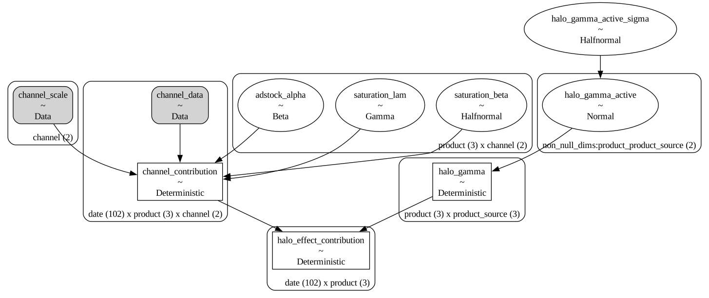
Rather than render the full computational graph, which apart from the halo term is the standard multi-dimensional MMM graph, we cut it down to the new pathway with var_names; the selected nodes bring their direct parents along. Read it bottom-up: MaskedPrior samples halo_gamma_active over the two active (receiver, source) pairs under the shared shrinkage scale halo_gamma_active_sigma, expands it to the full coefficient matrix halo_gamma with exact zeros on the inactive entries, and the effect multiplies that matrix onto the already-transformed channel_contribution to produce halo_effect_contribution, the term added to the mean.
pm.model_to_graphviz(
    mmm_flagship.model,
    var_names=[
        "halo_gamma_active_sigma",
        "halo_gamma_active",
        "halo_gamma",
        "halo_effect_contribution",
    ],
)
overlay_channel_contributions(
    mmm_flagship, "Channel contributions - flagship mask, sign-free"
);
Full spillover mask#
Every ordered pair is free. With three products that is six coefficients against 102 weeks, which is affordable. The point of fitting it is to see whether the extra freedom costs recovery on the pairs that are real, and to read off the asymmetry between flagship-to-small and small-to-flagship.
mmm_full = fit_halo_mmm(mask_full)
/var/folders/cm/3dzy9rdd5s3672z0s1brjkvh0000gn/T/ipykernel_75514/3212121386.py:40: UserWarning: This class is experimental and its API may change in future versions.
  gamma = MaskedPrior(prior, self.mask).create_variable(
NUTS[nutpie]: [y_sigma, adstock_alpha, saturation_lam, saturation_beta, halo_gamma_active_sigma, halo_gamma_active, intercept_contribution]
/Users/juanitorduz/Documents/pymc-marketing/.venv/lib/python3.14/site-packages/rich/live.py:260: UserWarning:
install "ipywidgets" for Jupyter support
  warnings.warn('install "ipywidgets" for Jupyter support')
/Users/juanitorduz/Documents/pymc-marketing/.venv/lib/python3.14/site-packages/rich/live.py:260: UserWarning:
install "ipywidgets" for Jupyter support
  warnings.warn('install "ipywidgets" for Jupyter support')
Sampling: [y]
/Users/juanitorduz/Documents/pymc-marketing/.venv/lib/python3.14/site-packages/rich/live.py:260: UserWarning:
install "ipywidgets" for Jupyter support
  warnings.warn('install "ipywidgets" for Jupyter support')
What a sign restriction costs#
Now the same flagship mask with a HalfNormal coefficient, the positive-only
prior used by most halo implementations, at the same hyperprior scale so the
comparison isolates the sign restriction. The DGP says product_c is
cannibalised at -0.5. A positive-only model cannot say that. The question is
what it says instead.
mmm_positive = fit_halo_mmm(
    mask_flagship,
    coefficient=Prior(
        "HalfNormal",
        sigma=Prior("HalfNormal", sigma=0.5),
        dims=("product", "product_source"),
    ),
)
/var/folders/cm/3dzy9rdd5s3672z0s1brjkvh0000gn/T/ipykernel_75514/3212121386.py:40: UserWarning: This class is experimental and its API may change in future versions.
  gamma = MaskedPrior(prior, self.mask).create_variable(
NUTS[nutpie]: [y_sigma, adstock_alpha, saturation_lam, saturation_beta, halo_gamma_active_sigma, halo_gamma_active, intercept_contribution]
/Users/juanitorduz/Documents/pymc-marketing/.venv/lib/python3.14/site-packages/rich/live.py:260: UserWarning:
install "ipywidgets" for Jupyter support
  warnings.warn('install "ipywidgets" for Jupyter support')
/Users/juanitorduz/Documents/pymc-marketing/.venv/lib/python3.14/site-packages/rich/live.py:260: UserWarning:
install "ipywidgets" for Jupyter support
  warnings.warn('install "ipywidgets" for Jupyter support')
Sampling: [y]
/Users/juanitorduz/Documents/pymc-marketing/.venv/lib/python3.14/site-packages/rich/live.py:260: UserWarning:
install "ipywidgets" for Jupyter support
  warnings.warn('install "ipywidgets" for Jupyter support')
gamma_free = mmm_flagship.idata.posterior["halo_gamma"].sel(
    product_source=FLAGSHIP, drop=True
)
gamma_pos = mmm_positive.idata.posterior["halo_gamma"].sel(
    product_source=FLAGSHIP, drop=True
)


def plot_cross_coefficients(
    estimates: dict[str, xr.DataArray],
    title: str,
    figsize: tuple[float, float] = (11, 5),
) -> Axes:
    """Forest plot of the receivers' cross coefficients, one colour per model.

    Each value of ``estimates`` is a posterior over the coefficient applied to
    the flagship's contribution, indexed by receiving product. The ground truth
    for each receiver is marked with a diamond.
    """
    labels = list(estimates)
    combined = xr.concat(
        [bare(da) for da in estimates.values()], dim="model"
    ).assign_coords(model=labels)

    pc = azp.plot_forest(
        xr.Dataset({"cross coefficient": combined.sel(product=RECEIVERS)}),
        combined=True,
        point_estimate="median",
        labels=["product"],
        figure_kwargs={"figsize": figsize, "layout": "constrained"},
    )
    pc.add_legend("model")
    ax = pc.viz["/"]["plot"].sel(column="forest").item()

    # One diamond per (receiver, model) row: the truth differs across receivers,
    # so a single vertical line would not do.
    point_estimate = pc.viz["point_estimate"]["cross coefficient"]
    is_first_marker = True
    for product in RECEIVERS:
        for label in labels:
            offsets = (
                point_estimate.sel(product=product, model=label).item().get_offsets()
            )
            ax.scatter(
                delta_true[PRODUCTS.index(product)],
                offsets[0, 1],
                color="black",
                marker="d",
                s=60,
                zorder=5,
                label="truth" if is_first_marker else None,
            )
            is_first_marker = False
    ax.axvline(0, color="gray", lw=0.8)
    # Both legends sit outside the data area: the model legend to the right of
    # the figure, the truth marker below the axes.
    ax.legend(loc="upper center", bbox_to_anchor=(0.5, -0.12))
    ax.set(xlabel="cross coefficient on the flagship contribution")
    ax.set_title(title, fontweight="bold")
    return ax


plot_cross_coefficients(
    {
        "flagship mask (Normal, sign-free)": gamma_free,
        "flagship mask (HalfNormal, positive only)": gamma_pos,
    },
    "A positive-only prior cannot report cannibalisation",
);
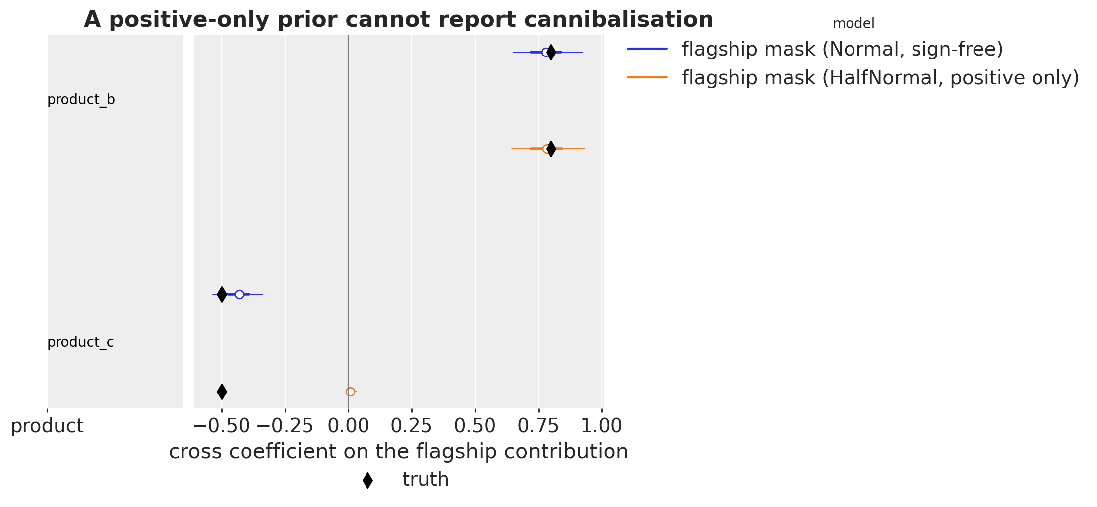
For product_b, where the truth is positive, the two priors agree almost
exactly: the restriction is invisible when it does not bind. For product_c
the failure is quiet, which is what makes it dangerous. The positive-only
posterior does not flag a problem, it simply concentrates near zero and reads
as “no meaningful spillover”. An analyst looking only at that model would
conclude the flagship is neutral for product_c, when in truth it is
actively costing it demand. The sign-free posterior recovers the negative
value.
This is the whole argument for making the cross coefficient sign-free by default, and it is independent of the adstock and saturation question.
Contrast: latent brand-awareness factor#
Mechanism 2 from the introduction. A single latent signal \(A_t = \sum_j w_j C_{t,j}\) driven by all products’ media, with product-specific sensitivities \(\lambda_i\). This is a rank-1 approximation \(\gamma_{ij} \approx \lambda_i w_j\): \(2P\) sampled parameters, of which \(2P - 1\) are identified because the weights are normalised to sum to one, instead of \(P(P-1)\).
It is structurally different from the masked matrix, not a variation on it: because \(w_j \ge 0\) and a single \(\lambda_i\) multiplies the whole factor, a product is either helped by the portfolio or hurt by it, uniformly. It cannot be lifted by one sibling and cannibalised by another. Here \(\lambda_i\) is sign-free so the model can at least express a uniformly negative sensitivity.
Note also that the rank-1 factor keeps its diagonal: product \(i\)’s own contribution enters its own awareness signal through \(w_i C_{t,i}\), so \(\lambda_i w_i\) competes with the own effect for the same signal. This is exactly the identifiability trap the masked matrix avoids by forcing the diagonal to zero, and it is part of why the factor’s posterior is wider than the masked estimates below.
class BrandAwarenessEffect(MuEffect):
    """Rank-1 latent brand-awareness factor shared across products."""

    prefix: str = "brand"
    product_dim: str = "product"
    sigma_lam: float = 0.5

    def create_data(self, mmm: MMM) -> None:
        """No extra data: the factor derives from channel_contribution."""

    def create_effect(self, mmm: MMM) -> XTensorVariable:
        """Build lambda_i * sum_j w_j * C_{t,j}."""
        total = mmm.model["channel_contribution"].sum(dim="channel")
        w_raw = pmd.HalfNormal("w_raw", sigma=1.0, dims=self.product_dim)
        w = pmd.Deterministic("w", w_raw / w_raw.sum(dim=self.product_dim))
        awareness = pmd.Deterministic(
            "brand_awareness", (w * total).sum(dim=self.product_dim)
        )
        lam_halo = pmd.Normal(
            "lam_halo", mu=0, sigma=self.sigma_lam, dims=self.product_dim
        )
        return pmd.Deterministic(
            f"{self.prefix}_effect_contribution",
            (lam_halo * awareness).transpose("date", ...),
        )

    def set_data(self, mmm: MMM, model: pm.Model, X: xr.Dataset) -> None:
        """No-op: the effect recomputes itself from the updated channel data."""


mmm_brand = MMM(
    date_column="date",
    channel_columns=CHANNELS,
    target_column="y",
    adstock=GeometricAdstock(l_max=L_MAX),
    saturation=LogisticSaturation(),
    dims=("product",),
)
mmm_brand.mu_effects.append(BrandAwarenessEffect())
mmm_brand.build_model(X, y)
mmm_brand.add_original_scale_contribution_variable(
    var=["channel_contribution", "brand_effect_contribution", "y"]
)
mmm_brand.fit(X=X, y=y, **SAMPLER_CONFIG)
mmm_brand.sample_posterior_predictive(X=X, random_seed=rng);
NUTS[nutpie]: [y_sigma, adstock_alpha, saturation_lam, saturation_beta, w_raw, lam_halo, intercept_contribution]
/Users/juanitorduz/Documents/pymc-marketing/.venv/lib/python3.14/site-packages/rich/live.py:260: UserWarning:
install "ipywidgets" for Jupyter support
  warnings.warn('install "ipywidgets" for Jupyter support')
/Users/juanitorduz/Documents/pymc-marketing/.venv/lib/python3.14/site-packages/rich/live.py:260: UserWarning:
install "ipywidgets" for Jupyter support
  warnings.warn('install "ipywidgets" for Jupyter support')
Sampling: [y]
/Users/juanitorduz/Documents/pymc-marketing/.venv/lib/python3.14/site-packages/rich/live.py:260: UserWarning:
install "ipywidgets" for Jupyter support
  warnings.warn('install "ipywidgets" for Jupyter support')
Recovery across approaches#
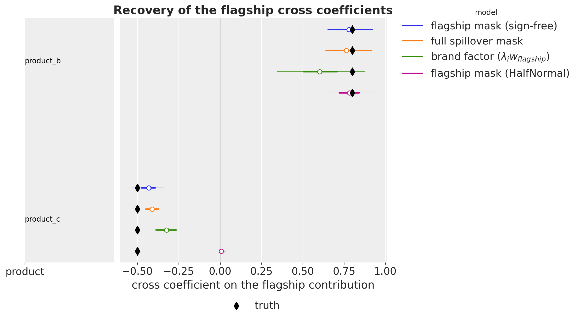
For each model we extract the implied coefficient on the flagship’s
contribution and compare against the truth. Comparing the scaled-space
coefficient directly against \(\delta\) relies on the target being scaled by a
single global constant, which is the MMM default; the assertion makes the
assumption explicit.
if mmm_flagship.idata.constant_data["target_scale"].size != 1:
    raise ValueError("The recovery plots assume a scalar (global max) target scale.")

gamma_full = mmm_full.idata.posterior["halo_gamma"].sel(
    product_source=FLAGSHIP, drop=True
)
w_flagship = mmm_brand.idata.posterior["w"].sel(product=FLAGSHIP, drop=True)
lam_brand = mmm_brand.idata.posterior["lam_halo"]

plot_cross_coefficients(
    {
        "flagship mask (sign-free)": gamma_free,
        "full spillover mask": gamma_full,
        "brand factor ($\\lambda_i w_{flagship}$)": lam_brand * w_flagship,
        "flagship mask (HalfNormal)": gamma_pos,
    },
    "Recovery of the flagship cross coefficients",
    figsize=(11, 6),
);
What predictive fit can and cannot tell you#
Before looking at the business quantity, it is worth checking what predictive
fit tells us. We score each model two ways, both in sample. The RMSE grades
only the posterior mean prediction. The
crps() grades the entire predictive
distribution against each observation, so a model that is right on average
but badly calibrated pays for it. CRPS is the stronger of the two, and it is
the most generous test we can give a purely in-sample metric.
models = {
    "baseline (no cross term)": mmm_baseline,
    "other products' spend as channel": mmm_other_spend,
    "flagship mask (sign-free)": mmm_flagship,
    "full spillover mask": mmm_full,
    "flagship mask (HalfNormal)": mmm_positive,
    "brand factor": mmm_brand,
}

y_target = np.zeros((n_dates_trimmed, N_PRODUCTS))
for ip, product in enumerate(PRODUCTS):
    y_target[:, ip] = data_df.loc[data_df["product"] == product, "y"].values


def in_sample_crps(mmm_obj: MMM, y_true: np.ndarray) -> float:
    """CRPS of the in-sample posterior predictive, on the original target scale."""
    predictive = (
        mmm_obj.idata.posterior_predictive["y"]
        * mmm_obj.idata.constant_data["target_scale"]
    )
    samples = predictive.stack(sample=("chain", "draw")).transpose(
        "sample", "date", "product"
    )
    return float(crps(y_true, samples.values))


fit_rows = []
for label, m in models.items():
    pp = m.idata.posterior_predictive["y"].values
    scale = m.idata.constant_data["target_scale"].values
    resid = (pp * scale).mean(axis=(0, 1)) - y_target
    # Diagnose convergence on the sampled free parameters only: the masked
    # gamma deterministic contains exact zeros whose r_hat is undefined.
    free_rv_names = [rv.name for rv in m.model.free_RVs]
    fit_rows.append(
        {
            "model": label,
            "in-sample RMSE": np.sqrt((resid**2).mean()),
            "in-sample CRPS": in_sample_crps(m, y_target),
            "max r_hat": float(
                az.summary(m.idata, var_names=free_rv_names)["r_hat"].max()
            ),
        }
    )

fit_table = pd.DataFrame(fit_rows).set_index("model")
fit_table.round(4)
| in-sample RMSE | in-sample CRPS | max r_hat | |
|---|---|---|---|
| model | |||
| baseline (no cross term) | 0.3152 | 0.1731 | 1.01 |
| other products' spend as channel | 0.2607 | 0.1450 | 1.01 |
| flagship mask (sign-free) | 0.2395 | 0.1308 | 1.01 |
| full spillover mask | 0.2369 | 0.1295 | 1.00 |
| flagship mask (HalfNormal) | 0.2595 | 0.1433 | 1.01 |
| brand factor | 0.2376 | 0.1297 | 1.01 |
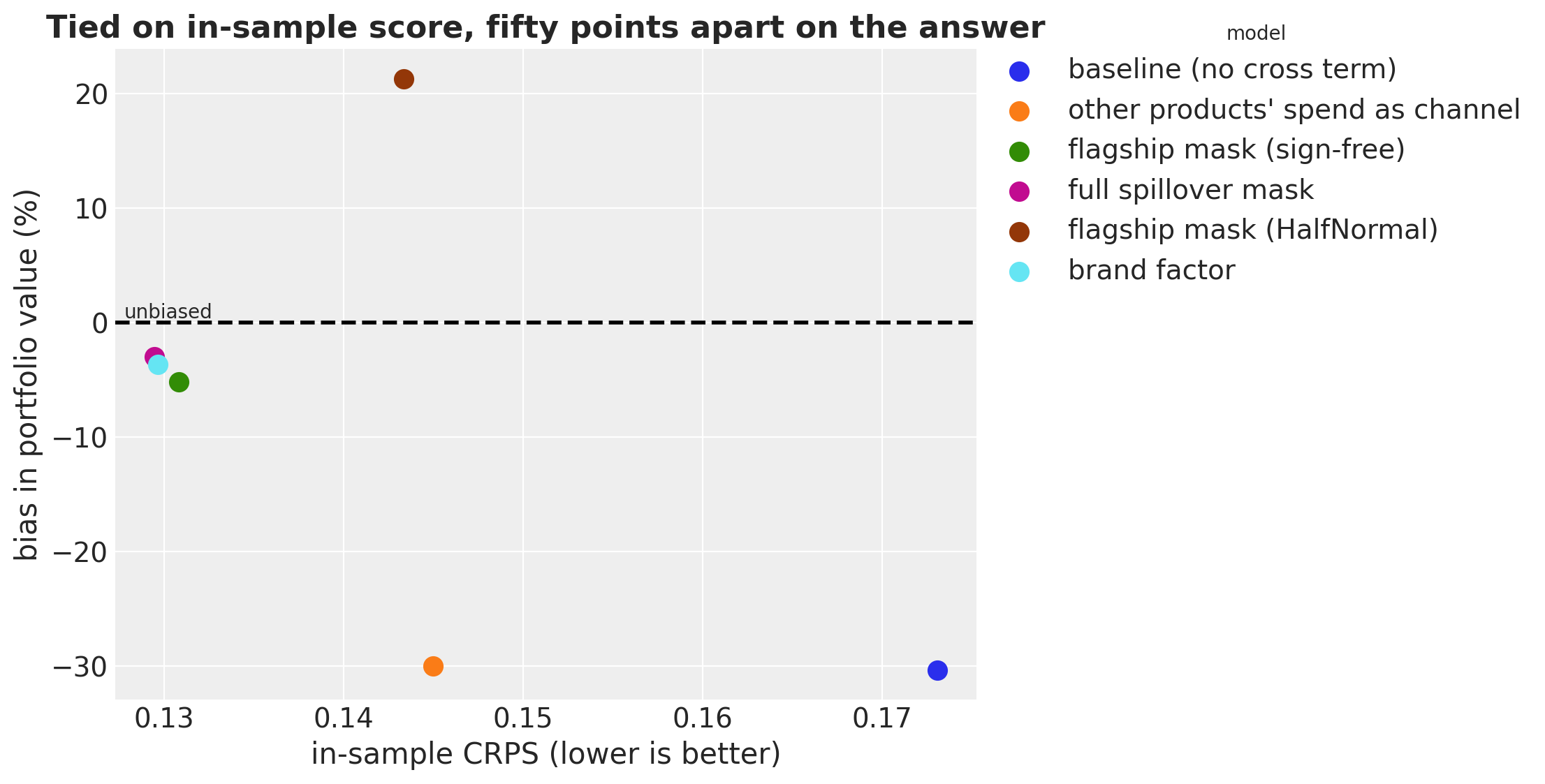
In-sample fit does notice that a mechanism is missing: the baseline, which
has no way to track the flagship-driven movement in product_b and
product_c, is the worst model on both scores. What fit cannot do is
choose among the models that carry some cross term. Every one of those sits
within about ten percent of the best RMSE and twelve percent of the best
CRPS, yet we will see below that the portfolio values they report span fifty
points, from thirty percent too low to twenty percent too high. Scoring the
whole predictive distribution rather than the mean does not rescue the
ranking, because the competing structures disagree about how to attribute a
signal they all reproduce equally well. This is the same lesson as
Funnel-Aware MMM: Upper to Lower-Funnel Mediation via a custom MuEffect: a structural bias shows up when you ask a causal
question, not in the loss curve. Do not select a halo structure on in-sample
fit.
The business quantity: portfolio-wide value of flagship media#
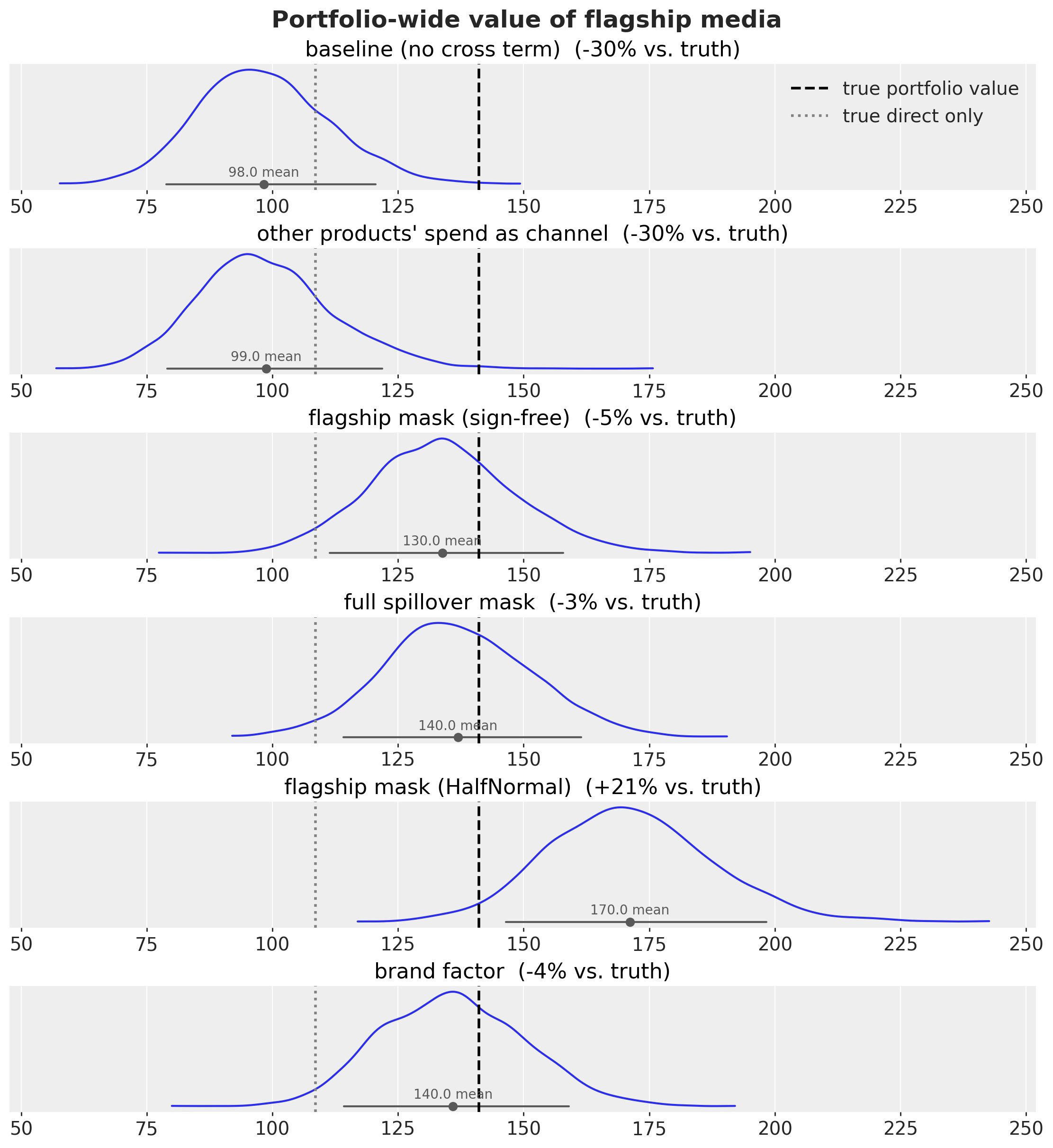
The decision this model exists to inform is how much the flagship’s media is worth across the portfolio, not just on its own line. In the DGP that is
The baseline has no cross term, so the best it could ever report is the direct term; the gap between that and the true portfolio value is the net cross effect it cannot see.
Each fitted model’s estimate of \(V\) must isolate the cross effects driven by the flagship: we multiply the model’s implied coefficient on the flagship (\(\gamma_{i,\text{flagship}}\) for the masked models, \(\lambda_i w_{\text{flagship}}\) for the brand factor) by the model’s estimate of \(C_{t,\text{flagship}}\). Summing a model’s whole cross-effect contribution would be wrong for the full mask, which also carries cross effects driven by the other products’ media. The baseline and the aggregate-spend workaround cannot attribute spillover to a source at all, so they report the direct term only.
true_direct = total_contribution_true_trimmed[:, FLAGSHIP_IDX].sum()
true_cross = halo_contribution_true_trimmed.sum()
true_portfolio = true_direct + true_cross

FLAGSHIP_GAMMA = {
    "flagship mask (sign-free)": lambda post: post["halo_gamma"].sel(
        product_source=FLAGSHIP, drop=True
    ),
    "full spillover mask": lambda post: post["halo_gamma"].sel(
        product_source=FLAGSHIP, drop=True
    ),
    "flagship mask (HalfNormal)": lambda post: post["halo_gamma"].sel(
        product_source=FLAGSHIP, drop=True
    ),
    "brand factor": lambda post: (
        post["lam_halo"] * post["w"].sel(product=FLAGSHIP, drop=True)
    ),
}

portfolio = {}

for label, m in models.items():
    post = m.idata.posterior
    flagship_contribution = (
        post["channel_contribution_original_scale"]
        .sel(product=FLAGSHIP, channel=CHANNELS, drop=True)
        .sum("channel")
    )
    direct = flagship_contribution.sum("date")
    implied_gamma = FLAGSHIP_GAMMA.get(label)
    cross = (
        (implied_gamma(post) * flagship_contribution).sum(("date", "product"))
        if implied_gamma
        else 0.0
    )
    portfolio[label] = bare(direct + cross)

portfolio_ds = xr.Dataset(portfolio)

pc = azp.plot_dist(
    portfolio_ds,
    col_wrap=1,
    figure_kwargs={
        "figsize": (11, 12),
        "sharex": True,
        "sharey": False,
        "layout": "constrained",
    },
)
fig = pc.viz["/"]["figure"].values.item()
for position, (ax, name) in enumerate(
    zip(fig.axes, portfolio_ds.data_vars, strict=True)
):
    ax.axvline(
        true_portfolio,
        color="black",
        linestyle="--",
        lw=2,
        label="true portfolio value",
    )
    ax.axvline(true_direct, color="gray", linestyle=":", lw=2, label="true direct only")
    bias = float(portfolio_ds[name].mean()) / true_portfolio - 1
    ax.set_title(f"{name}  ({bias:+.0%} vs. truth)")
    if position == 0:
        # The two reference lines are the same in every panel.
        ax.legend(loc="upper right")
fig.suptitle("Portfolio-wide value of flagship media", fontsize=18, fontweight="bold");
bias_table = pd.DataFrame(
    [
        {
            "model": label,
            "posterior mean": float(da.mean()),
            "bias vs. truth": float(da.mean()) / true_portfolio - 1,
        }
        for label, da in portfolio.items()
    ]
).set_index("model")
bias_table.assign(
    **{"bias vs. truth": lambda d: d["bias vs. truth"].map("{:+.1%}".format)}
).round(3)
| posterior mean | bias vs. truth | |
|---|---|---|
| model | ||
| baseline (no cross term) | 98.287 | -30.3% |
| other products' spend as channel | 98.746 | -30.0% |
| flagship mask (sign-free) | 133.807 | -5.2% |
| full spillover mask | 136.906 | -3.0% |
| flagship mask (HalfNormal) | 171.132 | +21.3% |
| brand factor | 135.921 | -3.7% |
Plotting the score against the answer shows how far an in-sample metric can be trusted. Read left to right, the ranking looks informative: the three models closest to the truth are also the three best on CRPS. Read vertically, it falls apart. The aggregate-spend workaround and the HalfNormal variant are separated by about one percent of CRPS and by fifty points of portfolio value, on opposite sides of the truth, so the score does not even carry the sign of the error you are about to make. And the sixteen percent CRPS improvement from the baseline to the workaround buys no reduction in bias at all.
fit_vs_bias = fit_table.join(bias_table["bias vs. truth"])

fig, ax = plt.subplots(figsize=(11, 5.5), layout="constrained")
for label, row in fit_vs_bias.iterrows():
    ax.scatter(row["in-sample CRPS"], 100 * row["bias vs. truth"], s=90, label=label)
ax.axhline(0, color="black", linestyle="--", lw=2)
ax.annotate("unbiased", xy=(0.01, 0), xycoords=("axes fraction", "data"), va="bottom")
fig.legend(loc="outside right upper", title="model")
ax.set(
    xlabel="in-sample CRPS (lower is better)",
    ylabel="bias in portfolio value (%)",
)
ax.set_title(
    "Tied on in-sample score, fifty points apart on the answer", fontweight="bold"
);
This table is the point of the notebook. The two models that cannot attribute
spillover to a source stop near the direct term, thirty percent short of the
truth. The two sign-free masked models land within about five percent. The
HalfNormal variant does not merely miss the cannibalisation, it converts the
missing loss into extra reported value: it keeps product_b’s halo, forces
product_c’s negative effect to zero, and comes out twenty percent above
the truth. An optimiser fed that number would over-fund the flagship, which
is the opposite failure to the one the baseline produces.
The brand factor lands close to the truth here, and it is worth being precise about why. This DGP has a single source with per-receiver signs, which is exactly a rank-1 matrix, and \(\lambda_i\) is sign-free per receiver, so the factor can represent this truth. Its posterior is nevertheless wider and pulled toward zero (see the recovery figure), because the diagonal terms compete with the own effects. Its bias is also not strictly comparable to the masked models’: the implied coefficient \(\lambda_i w_{\text{flagship}}\) is summed over every receiver including the flagship itself, so the diagonal term \(\lambda_a w_a\) enters the portfolio total, whereas the masked models have that entry fixed at zero and the DGP has no such term. With two sources of opposite sign acting on the same receiver it could not fit the truth at all.
Putting this into practice#
The simulation above is favourable: three products, a clean DGP, and a cross structure that one of the fitted masks matches exactly. Real portfolios are not like that. This section collects the checks that matter when the truth is unknown.
Choose the mask from business knowledge, then check it#
The mask is a set of claims about which pairs can interact, and it should come from people who know the portfolio: shared shelf space, shared audience, a launch calendar, a known flagship. Encoding a belief as a hard zero is stronger than encoding it as a tight prior, and it is also more honest, because it is falsifiable: if the business insists two products cannot interact and the model fits badly, that is information.
Start narrow and widen. A flagship mask that fits as well as a full mask is the better model, and the comparison costs one refit.
Between the flagship extreme (one known source) and the full-spillover
extreme (anything goes) there is a middle ground worth naming: product
similarity. Products that share an audience, a use case, or shelf space are
the plausible halo pairs; distant products are the plausible zeros. A
similarity or substitution matrix from category knowledge, survey data, or
purchase-switching data can be thresholded into a mask, or used more softly
as a per-pair prior scale so that similar pairs are allowed larger
coefficients. The same masked effect covers both variants: the mask carries
the hard zeros and the coefficient prior carries the soft structure.
Check identifiability before reporting a number#
A cross coefficient \(\gamma_{ij}\) and the receiver’s own channel coefficients both read a media-driven signal. When the two source signals are correlated, the posterior can trade one off against the other while leaving the fit unchanged. The diagnostic is the posterior correlation between them. If it is strongly negative, the pair is not separately identified and the right report is “not identified”, not a point estimate with a tight interval.
def cross_own_correlation(mmm_obj: MMM, receiver: str, source: str = FLAGSHIP) -> float:
    """Posterior correlation between a cross coefficient and the receiver's own beta."""
    post = mmm_obj.idata.posterior
    g = post["halo_gamma"].sel(product=receiver, product_source=source).values.flatten()
    own = post["saturation_beta"].sel(product=receiver).sum("channel").values.flatten()
    return float(np.corrcoef(g, own)[0, 1])


corr_table = pd.DataFrame(
    [
        {
            "receiver": p,
            "flagship mask": cross_own_correlation(mmm_flagship, p),
            "full spillover mask": cross_own_correlation(mmm_full, p),
        }
        for p in RECEIVERS
    ]
).set_index("receiver")
corr_table.round(3)
| flagship mask | full spillover mask | |
|---|---|---|
| receiver | ||
| product_b | 0.008 | 0.017 |
| product_c | 0.011 | -0.008 |
Here the correlations are close to zero, which is what a well-identified pair looks like: the spends were generated independently across products, so the flagship’s contribution and each receiver’s own media move separately, and the posterior does not need to trade one coefficient off against the other. In real portfolios, where campaigns are often planned on a shared calendar, expect worse.
The reason to expect worse is structural rather than statistical, and it is easier to see as a graph than as a correlation. Suppose an unobserved planning calendar \(K\) drives both products’ spend: a seasonal push, a joint retail event, a portfolio-wide budget cycle. Then \(C_A\) and \(y_B\) have a backdoor path through \(K\), and a cross coefficient fitted on \(C_A\) absorbs it. The model reports a halo, and nothing in the fit distinguishes that from a genuine transfer.
confounding = gr.Digraph()
confounding.attr(rankdir="LR")
confounding.attr("node", shape="ellipse")
confounding.node(
    "K", "planning calendar\n(K, unobserved)", color="black", style="dashed"
)
for node, label, style in [
    ("xa", "spend A", SPEND_STYLE),
    ("xb", "spend B", SPEND_STYLE),
    ("Ca", "C_A", CONTRIBUTION_STYLE),
    ("Cb", "C_B", CONTRIBUTION_STYLE),
    ("yb", "y_B", TARGET_STYLE),
]:
    confounding.node(node, label, **style)
confounding.edge("K", "xa")
confounding.edge("K", "xb")
confounding.edge("xa", "Ca")
confounding.edge("xb", "Cb")
confounding.edge("Cb", "yb", label="own effect")
confounding.edge("Ca", "yb", label="γ (halo?)", style="dashed", **HALO_STYLE)
confounding

The remedies are the ones that always apply to a backdoor path, not anything specific to halos: measure the calendar and control for it, so \(K\) stops being unobserved; or bring in variation that \(K\) does not touch, such as a lift test on the flagship. A cross-product term is a way to express transfer between products, not evidence that transfer is what produced the correlation. See Introducing causal discovery to PyMC-Marketing for the general treatment.
Read the asymmetry, it is usually the finding#
Under the full mask every ordered pair is free, so we can ask whether the flagship affects the smaller products more than they affect it. Asymmetry is typically the headline result of a halo study, and it is the thing a symmetric correlation analysis cannot deliver.
pairs = [(i, j) for i in PRODUCTS for j in PRODUCTS if i != j]
gamma_full_all = mmm_full.idata.posterior["halo_gamma"]

asym_rows = []
for i, j in pairs:
    da = gamma_full_all.sel(product=i, product_source=j)
    lo, hi = hdi_bounds(da)
    asym_rows.append(
        {
            "receiver": i,
            "source": j,
            "mean": float(da.mean()),
            "hdi 3%": float(lo),
            "hdi 97%": float(hi),
            "P(> 0)": float((da > 0).mean()),
        }
    )
asym_table = pd.DataFrame(asym_rows).set_index(["receiver", "source"])
asym_table.round(3)
| mean | hdi 3% | hdi 97% | P(> 0) | ||
|---|---|---|---|---|---|
| receiver | source | ||||
| product_a | product_b | -0.022 | -0.205 | 0.174 | 0.415 |
| product_c | 0.072 | -0.181 | 0.334 | 0.708 | |
| product_b | product_a | 0.769 | 0.618 | 0.938 | 1.000 |
| product_c | 0.224 | -0.035 | 0.459 | 0.957 | |
| product_c | product_a | -0.413 | -0.524 | -0.294 | 0.000 |
| product_b | -0.086 | -0.221 | 0.050 | 0.111 |
fig, ax = plt.subplots(figsize=(8, 6), layout="constrained")
mat = gamma_full_all.mean(("chain", "draw")).values
vmax = np.abs(mat).max()
im = ax.imshow(mat, cmap="RdBu_r", vmin=-vmax, vmax=vmax)
ax.grid(False)
ax.set_xticks(range(N_PRODUCTS), PRODUCTS, rotation=45, ha="right")
ax.set_yticks(range(N_PRODUCTS), PRODUCTS)
ax.set_xlabel("source $j$")
ax.set_ylabel("receiver $i$")
for a in range(N_PRODUCTS):
    for b in range(N_PRODUCTS):
        # Dark cells need light text.
        saturated = abs(mat[a, b]) > 0.6 * vmax
        ax.text(
            b,
            a,
            f"{mat[a, b]:+.2f}",
            ha="center",
            va="center",
            color="white" if saturated else "black",
        )
fig.colorbar(im, ax=ax, label="posterior mean $\\gamma_{ij}$")
ax.set_title(
    "Estimated cross-effect matrix (full mask)\nred = halo, blue = cannibalisation"
);
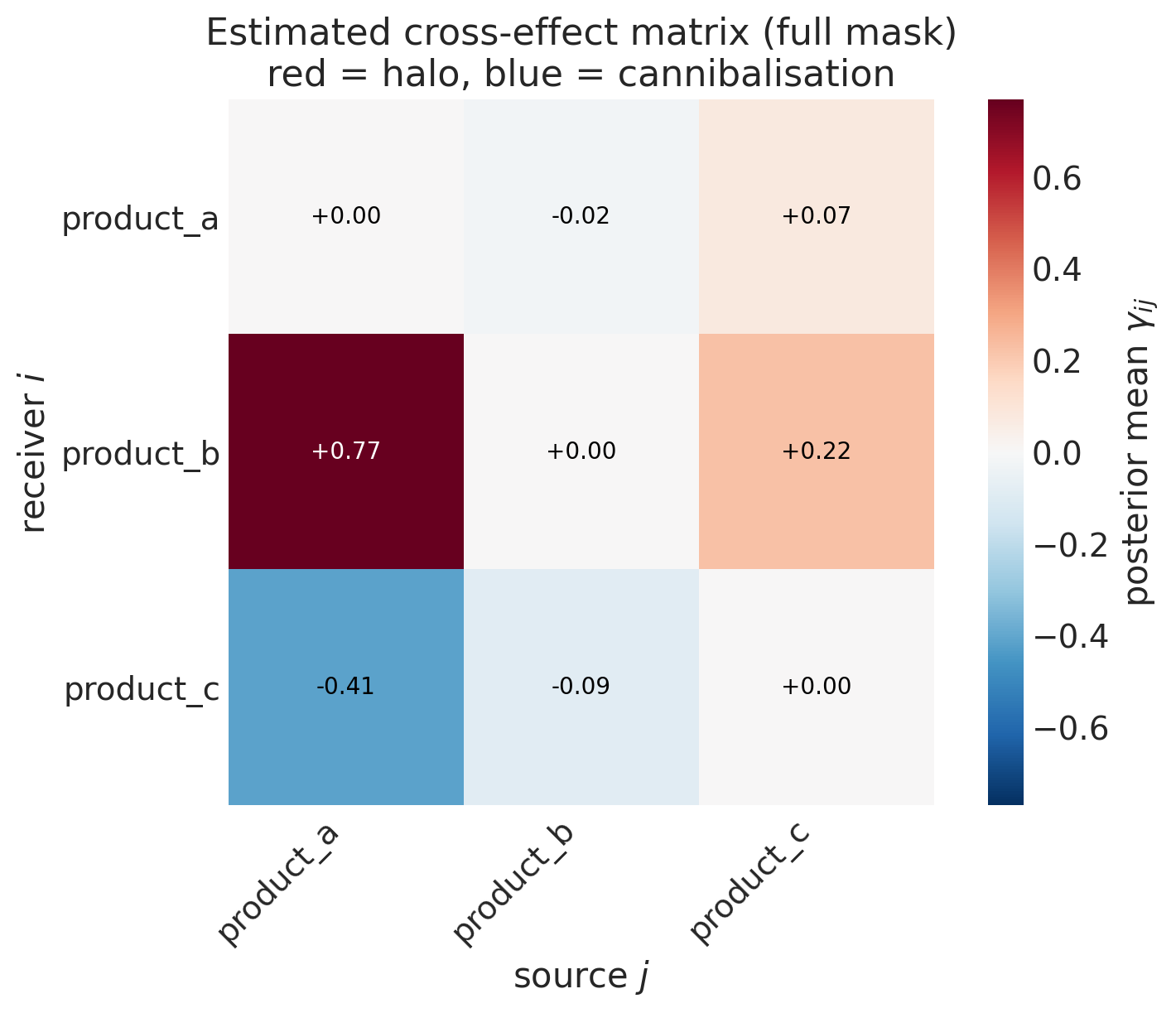
The flagship column carries the finding: a strong positive effect on
product_b and a clear negative effect on product_c, both with HDIs well
away from zero and covering the true values. Both point estimates are pulled
toward zero by the shrinkage hyperprior (\(0.769\) against \(0.8\), \(-0.413\)
against \(-0.5\)), which is the hyperprior working as intended rather than a
failure, but it is worth reporting the interval alongside the mean. The reverse direction, the
product_a row, is flat, which is the asymmetry a flagship story implies and
the thing a symmetric correlation analysis could not have delivered.
The cost of the full mask’s freedom is also visible. The
product_b ← product_c entry drifts positive with \(P(\gamma > 0)\) near
\(0.95\) even though its true value is zero: with six free coefficients and
correlated adstocked signals, one of the null pairs will absorb noise. The
flagship mask, which encodes the correct structure, has no room to produce
this artefact. That is the “start narrow and widen” advice made concrete.
Cap the total cross effect if the optimiser will consume it#
A model whose cross terms account for most of total media contribution is almost always over-attributing. A practical guardrail is to monitor the share of total media contribution carried by the cross term and treat a large share as a modelling failure rather than a finding.
true_cross_share = float(
    np.abs(halo_contribution_true_trimmed.sum())
    / (
        np.abs(channel_contribution_true_trimmed.sum())
        + np.abs(halo_contribution_true_trimmed.sum())
    )
)
print(f"true cross share: {true_cross_share:.3f}")
true cross share: 0.111
CROSS_VAR = {
    "flagship mask (sign-free)": "halo_effect_contribution_original_scale",
    "full spillover mask": "halo_effect_contribution_original_scale",
    "flagship mask (HalfNormal)": "halo_effect_contribution_original_scale",
    "brand factor": "brand_effect_contribution_original_scale",
}


def cross_share(mmm_obj: MMM, var: str) -> xr.DataArray:
    """Share of total media contribution carried by the cross term."""
    post = mmm_obj.idata.posterior
    own = post["channel_contribution_original_scale"].sum(
        ("date", "product", "channel")
    )
    cross = post[var].sum(("date", "product"))
    return np.abs(cross) / (np.abs(own) + np.abs(cross))


share_rows = []
for label, var in CROSS_VAR.items():
    s = cross_share(models[label], var)
    lo, hi = hdi_bounds(s)
    share_rows.append(
        {
            "model": label,
            "mean share": float(s.mean()),
            "hdi 3%": float(lo),
            "hdi 97%": float(hi),
        }
    )
pd.DataFrame(share_rows).set_index("model").round(3)
| mean share | hdi 3% | hdi 97% | |
|---|---|---|---|
| model | |||
| flagship mask (sign-free) | 0.128 | 0.077 | 0.183 |
| full spillover mask | 0.158 | 0.073 | 0.257 |
| flagship mask (HalfNormal) | 0.245 | 0.201 | 0.290 |
| brand factor | 0.115 | 0.000 | 0.248 |
The flagship mask sits close to the true share of \(0.111\) computed above, and the brand factor is close too, though with an interval running down to zero. The full mask overshoots by about forty percent: the extra free pairs each carry a little noise and the shares add up. The HalfNormal variant carries more than twice the true share: deleting the negative entry inflates the net cross term, the same over-attribution seen in the portfolio table.
Remaining caveats#
A coefficient is a net. Nothing here separates a simultaneous halo and cannibalisation between the same pair. That needs channel-resolved sources.
Scale. At \(P\) in the tens, even a masked matrix needs the shrinkage hyperprior to be doing real work. Check that the estimated scale is small and that widening the mask does not simply inflate it.
Confounding. If two products are advertised on correlated calendars, a cross coefficient will happily absorb the common cause. Cross-product terms do not repair a missing confounder, and the usual remedies (controls, lift tests, an explicit causal graph) still apply. See Introducing causal discovery to PyMC-Marketing.
Feedback. The model is a one-step transfer. Genuine mutual reinforcement over time is a dynamic system and is not what this parameterisation estimates.
Conclusion#
Put the cross term on the already-transformed contribution \(C_{t,j}\) and apply a plain linear coefficient. Transform once, read linearly many times. A cross term on raw spend with no saturation grows without bound and will mislead a budget optimiser.
Make the coefficient sign-free. Halo and cannibalisation are one parameter with two signs, and a positive-only prior does not fail loudly, it reports “no effect” for a cannibalised product.
Use a mask to encode which pairs may interact, and a shrinkage hyperprior to keep the surviving coefficients honest. One masked effect covers the flagship, full-spillover, block and hierarchy structures.
Do not select on predictive fit. In-sample error notices a missing mechanism at best. Scoring the full predictive distribution with CRPS does not help: the two structures whose portfolio values are fifty points apart, on opposite sides of the truth, sit within about one percent of each other on in-sample CRPS.
Identification comes from variation. The cross coefficient is read off the temporal variation of the source’s transformed contribution. A flagship parked deep in saturation offers none, and no prior can rescue that.
Report identifiability alongside the estimate. When a cross coefficient and the receiver’s own effect are strongly anti-correlated in the posterior, the honest answer is that the pair is not separately identified.
%load_ext watermark
%watermark -n -u -v -iv -w -p pymc_marketing,pytensor
Last updated: Wed, 12 Aug 2026

Python implementation: CPython
Python version       : 3.14.2
IPython version      : 9.15.0

pymc_marketing: 1.0.0
pytensor      : 3.0.7

arviz         : 1.2.0
arviz_plots   : 1.2.0
graphviz      : 0.21
matplotlib    : 3.10.9
numpy         : 2.4.6
pandas        : 2.3.3
pydantic      : 2.13.4
pymc          : 6.0.1
pymc_extras   : 0.12.2.dev1+gee8cc37df
pymc_marketing: 1.0.0
pytensor      : 3.0.7
xarray        : 2026.4.0

Watermark: 2.6.0