

Advanced Funnel-Aware MMM: Geo-Level Mediation Through Lower-Funnel Spend#
The Funnel-Aware MMM: Upper to Lower-Funnel Mediation via a custom MuEffect notebook introduced the core idea. Upper-funnel activity creates demand, and that demand shows up later in lower-funnel channels. A custom MuEffect with its own likelihood encodes that mediation directly in the model. That example kept the funnel deliberately minimal: one upper channel, one mediator, one national time series. Real applications are not that tidy. This notebook scales the same idea up to a setup that looks much more like production work.
Executive summary#
The question. Upper-funnel media creates demand that later converts through lower-funnel spend. A media mix model can treat that lower-funnel spend as just another channel, leave it out, or control for a symptom of demand instead. What happens to its ROAS estimates in each case?
The setup. A synthetic weekly geo panel with a known ground truth. It has two upper-funnel channels (tv_spend, social_spend) and a lower-funnel mediator that is itself paid media (lower_spend). A branded-search series (search_volume) tracks demand but causes nothing. The media plans are confounded with category demand through a seasonal cycle, a growth trend, and correlated noise.
The contenders. Six models are fit to the same data. Five are naive specifications, Naive A through Naive C, and each mishandles the funnel in a characteristic way. The sixth is the funnel model, which encodes the mediation explicitly through a custom MuEffect. The section Model structures we will study below defines each one before any code runs.
The decision. Measurement is only half of the job. At the end we put the fitted funnel model through the budget optimizer, in-sample: same total weekly budget, \(\pm 50\%\) per geo \(\times\) channel cell, the historical spend pattern kept fixed. We run it twice on the same posterior. One run uses the library’s default objective, which scores the direct path only. The other uses total_response_original_scale, which also counts the demand the media create downstream. We check both plans against the known truth. The section also lists what a custom effect needs before the optimizer can price the mediated path, and it verifies each requirement at run time.
The punchlines.
A bit over a third of each upper channel’s true effect travels through the mediator. A model that cannot see the funnel has to put that mass somewhere. Where it lands is a property of the likelihood, not something a correlation table can tell you in advance.
All six models fit the target almost equally well: they span less than a point of in-sample \(R^2\). Their ROAS conclusions still differ by tens of percent. Predictive fit does not diagnose causal bias. The Nürnberger Versicherung case study, which faced this same funnel problem in production, put it well:
“Trust is not created by \(R^2\) values. It is created when business reality matches model expectations.” (Philip Herp, Nürnberger Versicherung)
The funnel model is the only specification that covers the true total ROAS in all six geo-channel cells, and it also has the narrowest intervals. Every naive model fails differently.
Naive Aanswers a different question (the direct effect).Naive Bis confounded and misallocates the mediated demand pool. The two “fixed” variants repair only the channel that was materially confounded.Naive Cblocks part of the very effect it is trying to measure.A formal d-separation analysis predicts most of this before any model is fit. The one place where the graph’s ranking and the data disagree is itself instructive: a valid adjustment set says which variables you need, never how they must enter the model.
The budget optimizer prices the funnel only if you tell it to. Its default objective scores the direct path alone. At the historical plan that is 68.2% of the media-driven response under the posterior (61% in truth). Per cell, the default objective sees between 56% and 72% of the marginal response the decision turns on. The funnel-aware objective,
total_response_original_scale, agrees with the default on the direction of five of six moves and moves two cells by about ten points. It also flips the sign ofsouth, tv_spend. ThenorthandsouthTV cells have the same direct marginal response, butsouth’s mediated marginal is twicenorth’s. It creates more demand per unit of spend, and its lower funnel converts that demand at a steeper point of the shared curve. On this dataset the funnel-aware plan is worth more on the generative truth: +0.51% against +0.36% in media-driven response, gross of the extra lower-funnel spend the new demand induces. The uplifts are small (about 1%) because the synthetic plan was already close to the posterior optimum within the bounds. The true uplifts sit inside the posterior intervals.
The route. The causal graph comes first, then the model definitions and the data-generating process. A d-separation analysis of every specification follows, then the six fits. The comparisons close the measurement half: parameter recovery, effect decompositions, ROAS with bias and coverage tables, and what the built-in decomposition can and cannot see. One built-in does follow the funnel: the custom effect opts in through incrementality_spec, so the ROAS totals come from the incrementality module, which follows the per-channel spend counterfactual down both paths. The last section, Funnel-aware budget optimization, turns the fitted model into a budget decision.
Five things make this example “advanced”:
Several upper-funnel channels feed the same latent demand pool, each with its own carryover and saturation.
A geo panel: the model is fit across regions at once, with some parameters pooled across geos and others estimated per geo.
A mediator that is itself media. Lower-funnel spend is not a passive symptom of demand; it is paid search, and it converts. It sits on the causal path. The demand that upper-funnel activity creates drives part of it, and an exogenous budget of its own drives the rest.
A second, purely observational proxy. Branded search volume measures the same latent demand but causes nothing. Keeping a cause and an indicator distinct is most of the modeling problem.
Confounded media plans. Category demand and the media plans share an annual seasonal cycle, a growth trend (materially for one channel only), and a small amount of correlated noise. Every model absorbs the seasonal strand through its Fourier basis. The trend strand is just as observable, but none of the standard specifications carries it. The noise strand is observable by nobody. The causal analysis below is organised around that three-way split, and around what fixing each strand does and does not buy.
Two pieces of the library keep the code short. DataVarMuEffect feeds the effect its data, so we only write the part of the effect that is genuinely custom. pymc.dims xtensors give named broadcasting, so a ("geo",) parameter, a ("channel",) parameter and a ("date", "geo", "channel") data array combine without a single reshape. Before we fit anything, we interrogate the causal graph itself with networkx. For every adjustment-based specification we compute, rather than assert, whether it identifies the effect it claims to.
The funnel structure#
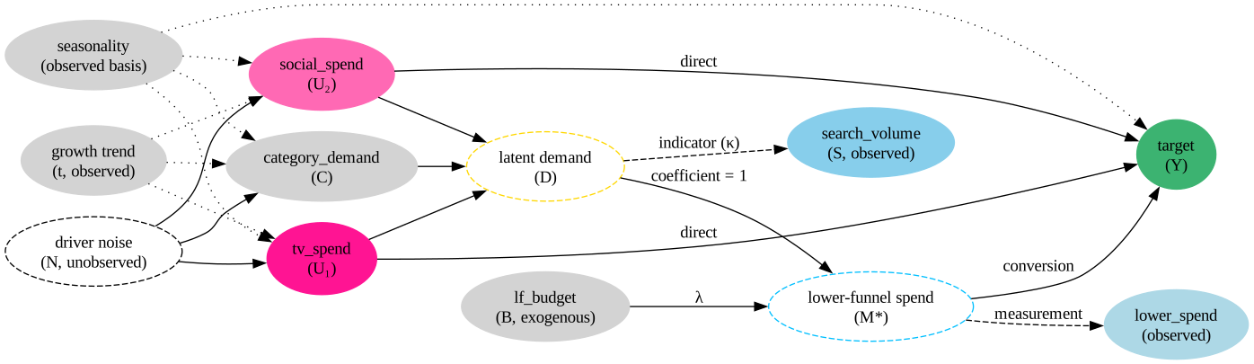
We model a weekly geo panel. Every model in this notebook is, at heart, a claim about which causal arrows exist between media, demand, and sales, so we start from the graph itself. The figure below is the reference point for everything that follows:
Tip
How to read the figure. Filled nodes are observed: they appear in a dataset. A dashed outline marks the three quantities no dataset contains (\(D\), \(M^{*}\) and \(N\)). Dotted arrows are deterministic calendar components. Dashed arrows are measurement or indicator links, not causal ones. Solid arrows are ordinary structural edges.
The nodes, from media to target. Within every geo \(g\) and week \(t\):
tv_spend,social_spend(\(U_{t,g,c}\)): two upper-funnel channels.category_demand(\(C_{t,g}\)): an exogenous, seasonal index of how much the whole category is in-market (think a category-level search-trend index). It drives lower-funnel demand but does not act on the target directly. That missing arrow is an exclusion restriction on the mediator equation.lf_budget(\(B_{t,g}\)): an exogenous lower-funnel budget of always-on spend plus promotional pushes. The search team sets it on its own calendar, not in response to demand.\(D_{t,g}\): latent demand. Never observed.
\(M^{*}_{t,g}\): structural lower-funnel spend, the quantity that actually buys conversions.
lower_spendis this observed with reporting noise.search_volume(\(S_{t,g}\)): branded search volume, an indicator of \(D\).y(\(Y_{t,g}\)): the target.
The arrows in the figure are these four equations. Upper-funnel activity and the category cycle create demand:
That demand is one of two things the search team’s spend responds to; the other is its own budget. Both parts are real money and both convert:
Branded search, by contrast, buys nothing. It is a pure indicator; people search for the brand because they are in-market:
Finally the target responds to lower-funnel spend, plus the direct effect of each upper channel and its own seasonality:
Every upper channel therefore reaches the target along two paths: directly, and indirectly along \(U \to D \to M^{*} \to Y\).
Two details of the drawing carry real modeling weight.
\(M^{*}\) and lower_spend are two nodes on purpose. What a dataset carries is the filled node, at the other end of the dashed measurement edge. The gap between the structural quantity and its noisy observation is what makes Naive A an approximate rather than an exact direct-effect estimator below.
The market driver appears three times, and only two of the three are observed. seasonality is the annual cycle, a deterministic function of the calendar that every model below matches with a Fourier basis. t is the common growth trend in the plans and the category index. The trend is equally deterministic and equally observable, but it sits outside the span of an annual basis, so the shared Fourier term cannot stand in for it. N is the drivers’ shared noise, the one strand that is genuinely unobserved. It is small but not zero, and we measure it explicitly once the covariates are drawn.
Splitting the driver up is not cosmetic. The three strands have completely different statuses in the models below. Every specification conditions on the season by construction. Only the models that add a control on purpose carry the trend. Nothing can condition on \(N\). Conflating the three under a single “seasonality” bubble is precisely how the confounding in Naive B stays invisible. And, as the d-separation table will show, dropping \(N\) from the picture certifies a specification that should only have been certified conditionally. A confounder does not have to be unobservable to bite; it only has to be missing from the regression.
Note
\(N\) is not a device invented for the picture. The covariate simulation below gives the two media plans and the category index a shared error term (pm.LKJCholeskyCov). For d-separation purposes that is equivalent to an unobserved common cause of all three. (A single latent is a rank-one stand-in for a general \(3 \times 3\) correlation; splitting \(N\) into three pairwise causes changes none of the verdicts below.) The correlation is small, and we measure it once the covariates exist. But drawing it changes the d-separation verdicts, so it belongs on the graph.
Why only one of the two downstream variables points at the target#
This asymmetry is the heart of the example, so it is worth stating bluntly.
Lower-funnel spend belongs in the target equation. It is paid media. Money goes in, conversions come out, and a model that leaves it out is missing a real driver. What makes it a mediator rather than an ordinary channel is that its level is not chosen freely. Part of it responds to demand that upper-funnel activity created, and credit for that part belongs upstream.
Branded search volume does not. Nobody buys search volume; it is a symptom of being in-market. Drawing \(S \to Y\) would invent a causal channel that does not exist. As Naive C below demonstrates, putting it into an MMM as if it were a channel silently blocks the very path we are trying to measure.
Important
The practical test is not “is this variable predictive of sales?” Both are, very. It is “if I doubled it, would sales move?” That question separates a spend line from a tracking metric, and no amount of model fit will answer it for you.
Note
What anchors the latent scale. \(D\) is latent, so something has to fix its units. Here the coefficient on \(D\) in the \(M^{*}\) equation is pinned at exactly one: latent demand is measured in units of the lower-funnel spend it induces. Everything else is then relative to that. \(\kappa\) is free, and \(\lambda\) converts budget into the same units. Were that coefficient free too, rescaling \(D\) and compensating in \(\kappa\) would leave the likelihood untouched.
Two further structural features make this harder than the single-channel case.
Confounded media plans. Media plans and category demand are built around the same market rhythm, so upper-funnel spend and category demand move together. That common cause has three strands, with very different statuses relative to the models below:
The purely seasonal strand is a deterministic function of the calendar. Every model below includes the matching Fourier basis, so this strand is adjusted for by construction, however large it looks in a correlation table.
The TV plan and the category index also share a strong common growth trend. The trend is observable from the calendar just as the season is, yet it sits outside the span of a smooth annual basis, so a Fourier term cannot absorb it. Only the models that deliberately control for it touch that strand:
Naive B+through the category index,Naive B++through the trend itself.The third strand is the drivers’ shared noise, which no regressor spans and no control column can reach. It is small here. But small is a measurement, not an assumption, and the d-separation verdicts turn out to depend on it.
We will measure how much confounding each strand is actually worth before fitting anything. Then we watch the models separate what adjustment can repair from what it cannot. The trend-driven part of category demand is removable by adjustment; the demand each channel creates downstream is not. Which curve collects what is decided by the likelihood’s fit, not by anything a correlation table can tell you in advance.
A shared, saturating demand pool. Because both channels push on the same saturating function, their indirect effects are not additive. Turning off TV alone and turning off social alone remove less demand between them than turning off both at once. Each channel is partly shielded by the other’s contribution sitting further along the concave curve. We quantify this below.
Identification rests on two exclusion restrictions (two arrows deliberately missing from the graph), and they are not equally load-bearing:
The lower-funnel budget \(B\) enters the spend equation but not the search equation. This one is genuinely identifying: it lets the model tell \(\lambda B\) apart from \(D\) rather than lumping the two into one unidentified level. Nothing else in the model can substitute for it.
Category demand \(C\) enters the demand equation but not the target. This one is a modelling convenience rather than a necessity. \(C\) is observed, so a direct \(C \to Y\) path could simply be absorbed by adding \(C\) as a control column. Keeping the target equation clean makes the example sharper, but no identification would be lost by relaxing it, a fact
Naive B+below exploits.
The whole graph is replicated across geos. Which parameters are shared and which are free per geo is a modeling choice, and with roughly 130 weeks per geo it is a consequential one:
Parameter |
Dimensions |
Why |
|---|---|---|
|
|
Carryover and curvature are properties of the medium, not the region; pooling them buys a lot of precision. |
|
|
Response amplitude genuinely differs by region (market size, competition). |
|
|
Regional levels and volatility; how strongly budget converts into spend is a regional operating choice. |
|
|
The conversion path from lower-funnel spend to the target: how fast paid-search clicks convert and how hard they saturate is a property of each regional market. |
|
scalar |
There is only one mediator, so unlike |
|
scalar |
The search index is the same instrument everywhere, so its loading is shared. |
Mixing pooled and unpooled parameters in one expression is where xtensors earn their keep. pymc.dims aligns operands by dimension name, so a ("channel",) decay multiplies a ("date", "geo", "channel") media array with no manual broadcasting.
Model structures we will study#
The comparisons below are organised around six model structures, so let us define them before any code runs. Every one is a geo-level MMM with the same adstock/saturation families, the same priors, the same Fourier seasonal basis, and the same sampler settings. The two upper-funnel channels are always present. The models differ in exactly one thing: what else they condition on, and how.
Model |
Beyond the two upper channels |
How it treats the funnel |
Question it can answer |
|---|---|---|---|
|
adds |
conditions on the mediator, which blocks the indirect path |
approximately the direct effect of the upper channels |
|
nothing |
ignores the mediator entirely |
targets the total effect, but a backdoor through the shared market driver stays open |
|
adds |
still ignores the mediator, but blocks that backdoor through the observed demand index |
the total effect: formally valid |
|
adds the growth trend |
blocks only the trend strand of the backdoor; the drivers’ shared noise stays open |
the total effect: valid only conditionally |
|
adds |
conditions on a symptom of demand, partially blocking the indirect path |
neither effect cleanly |
|
the |
models the mediation explicitly |
direct, indirect and total, separately |
The comparison tables and figures below print these labels verbatim. The prose uses the full form whenever a model is (re)introduced, so a name never has to be held in memory across sections. The short forms Naive A through Naive C appear inside a discussion that has already named the model in full, and as row labels in the compact diagnostic tables. The d-separation section below computes the causal verdicts sketched in the last column. The fitting section then tests them against the known ground truth. Only the Funnel model goes on to the budget optimization at the end. The point there is not another model comparison but what the same fitted model recommends under two objectives, one blind to the mediated path and one that prices it.
Prepare Notebook#
import itertools

import arviz as az
import arviz_plots as azp
import matplotlib.pyplot as plt
import networkx as nx
import numpy as np
import pandas as pd
import pymc as pm
import pymc.dims as pmd
import pytensor
import pytensor.tensor as pt
import xarray as xr
from pydantic import InstanceOf
from pymc import do
from pymc_extras.prior import Prior
from pytensor.graph import rewrite_graph

from pymc_marketing.mmm import GeometricAdstock, LogisticSaturation
from pymc_marketing.mmm.additive_effect import DataVarMuEffect, IncrementalitySpec
from pymc_marketing.mmm.budget_optimizer import BudgetOptimizer
from pymc_marketing.mmm.media_transformation import MediaTransformation
from pymc_marketing.mmm.mmm import MMM

az.style.use("arviz-darkgrid")
plt.rcParams["figure.figsize"] = [10, 6]
plt.rcParams["figure.dpi"] = 100
plt.rcParams["figure.facecolor"] = "white"

%config InlineBackend.figure_format = "retina"
seed: int = sum(map(ord, "geo funnel model"))
rng: np.random.Generator = np.random.default_rng(seed=seed)
Configuration#
n_dates = 130
l_max = 8
geos = ["north", "south", "west"]
channels = ["tv_spend", "social_spend"]

date_range = pd.date_range(start="2021-01-04", freq="W-MON", periods=n_dates)
coords = {"date": date_range, "geo": geos}
The FunnelEffect component#
A MuEffect adds an arbitrary term to the target mean through a three-method protocol. create_data registers the data the effect needs. create_effect builds and returns the term. set_data refreshes the data at prediction time. create_effect runs inside the model context, so it can declare its own observed likelihoods. That is what turns “add a term to mu” into “fit extra structural equations jointly”.
DataVarMuEffect removes most of that boilerplate, and both this notebook and Funnel-Aware MMM: Upper to Lower-Funnel Mediation via a custom MuEffect build on it. It takes a list of data_vars naming variables in the training dataset and implements create_data and set_data for us. Each variable keeps the dimensions it already carries in the dataset, which is also what makes the effect work out of sample.
What is new here is one level up. The MediaTransformation helper does for the adstock/saturation pairs what DataVarMuEffect does for the data. The basic notebook’s effect carries four loose components; this one holds two transformation objects. Each pair is ordered by a single adstock_first flag, and every component’s priors carry their own dimensions. That matters here because every prior in the geo panel needs dimensions attached to it.
One more method matters for the ROAS section later. The effect reads mmm.channel_data_scaled, so a spend counterfactual reaches the target through it as well as through channel_contribution. Returning an IncrementalitySpec from incrementality_spec declares exactly that. Without the declaration, the incrementality module refuses to run rather than quietly report the direct path as if it were the total. The mediator chains a second adstock behind the model’s own, so a spend change can travel extra weeks downstream. The declaration records that reach, and the yearly evaluation windows below are sized by it.
What remains in create_effect is exactly the part that is the funnel:
class FunnelEffect(DataVarMuEffect):
    """Geo-level upper-funnel mediation through lower-funnel spend.

    Encodes ``upper channels -> latent demand -> lower-funnel spend -> target`` as
    an additive effect on the target mean, while jointly fitting the observed
    lower-funnel spend and an indicator of the latent demand.
    """

    upper_transform: InstanceOf[MediaTransformation]
    demand_transform: InstanceOf[MediaTransformation]

    model_config = {"arbitrary_types_allowed": True}

    def to_dict(self) -> dict:
        """Serialize the effect (transformations delegate to their own dicts)."""
        return {
            "data_vars": self.data_vars,
            "prefix": self.prefix,
            "upper_transform": self.upper_transform.to_dict(),
            "demand_transform": self.demand_transform.to_dict(),
        }

    def incrementality_spec(self) -> IncrementalitySpec:
        """Opt in to incrementality, declaring the second adstock's reach.

        A spend counterfactual moves this contribution because it reads
        ``mmm.channel_data_scaled``; opting in tells the incrementality module
        to include that movement in the increment. The mediator chains a
        second adstock behind the model's own, so a change in spend can still
        move this contribution up to ``demand_transform.adstock.l_max`` weeks
        beyond the base ``l_max``; declaring it sizes the evaluation windows
        for the yearly breakdown below. (The empty ``IncrementalitySpec()``
        also works, the reach is then measured off the fitted graph, as the
        basic funnel notebook does, but a declaration this cheap is worth
        writing down.)
        """
        return IncrementalitySpec(
            additional_carryover_lags=self.demand_transform.adstock.l_max
        )

    def create_effect(self, mmm):
        """Build the mediator equation, its likelihoods, and the target effect."""
        model = mmm.model

        # ("date", "geo", "channel") -> ("date", "geo"): every upper channel
        # pushes on the same demand pool, so we sum the channel dimension away.
        upper_on_demand = self.upper_transform(mmm.channel_data_scaled, dim="date").sum(
            dim="channel"
        )

        # Structural equation 1: upper spend + category demand -> latent demand.
        baseline = pmd.HalfNormal(f"{self.prefix}_baseline", sigma=1.0, dims=("geo",))
        gamma = pmd.HalfNormal(f"{self.prefix}_gamma", sigma=1.0, dims=("geo",))
        demand = pmd.Deterministic(
            f"{self.prefix}_demand",
            baseline + gamma * model["category_demand"] + upper_on_demand,
        )

        # Structural equation 2: lower-funnel spend responds to demand (coefficient
        # fixed at 1, which anchors D's scale) and to its own exogenous budget.
        lam_b = pmd.HalfNormal(f"{self.prefix}_lambda", sigma=0.5, dims=("geo",))
        lf_spend = pmd.Deterministic(
            f"{self.prefix}_lf_spend",
            demand + lam_b * model["lf_budget"],
        )

        # Observation: reported lower-funnel spend, up to reporting noise.
        pmd.TruncatedNormal(
            f"{self.prefix}_lower_spend_likelihood",
            mu=lf_spend,
            sigma=pmd.HalfNormal(f"{self.prefix}_sigma_m", sigma=1.0, dims=("geo",)),
            lower=0.0,
            observed=model["lower_spend"],
        )

        # Indicator: branded search volume loads on demand, not on spend.
        kappa = pmd.HalfNormal(f"{self.prefix}_kappa", sigma=1.0)
        pmd.Normal(
            f"{self.prefix}_search_likelihood",
            mu=kappa * demand,
            sigma=pmd.HalfNormal(f"{self.prefix}_sigma_s", sigma=1.0, dims=("geo",)),
            observed=model["search_volume"],
        )

        # Structural equation 3: lower-funnel spend -> target contribution.
        return pmd.Deterministic(
            f"{self.prefix}_effect_contribution",
            self.demand_transform(lf_spend, dim="date"),
        )
The factory below wires up the two transformations and, crucially, sets the dimensions of each prior according to the pooling table above. GeometricAdstock and LogisticSaturation accept a priors dictionary, so alpha and lam get dims="channel" (pooled across geos) while beta gets dims=("geo", "channel"). Unique prefix values keep these parameters from colliding with the base MMM’s own direct-path transforms.
def make_funnel_effect() -> FunnelEffect:
    """Construct the funnel effect with uniquely-prefixed transformations."""
    return FunnelEffect(
        data_vars=["lower_spend", "search_volume", "category_demand", "lf_budget"],
        prefix="funnel",
        upper_transform=MediaTransformation(
            adstock=GeometricAdstock(
                l_max=l_max,
                prefix="adstock_uf",
                priors={"alpha": Prior("Beta", alpha=2, beta=3, dims="channel")},
            ),
            saturation=LogisticSaturation(
                prefix="sat_uf",
                priors={
                    "lam": Prior("Gamma", mu=2.0, sigma=1.0, dims="channel"),
                    "beta": Prior("HalfNormal", sigma=1.0, dims=("geo", "channel")),
                },
            ),
            adstock_first=True,
            dims=("geo", "channel"),
        ),
        demand_transform=MediaTransformation(
            adstock=GeometricAdstock(
                l_max=l_max,
                prefix="adstock_lf",
                priors={"alpha": Prior("Beta", alpha=2, beta=3, dims="geo")},
            ),
            saturation=LogisticSaturation(
                prefix="sat_lf",
                priors={
                    "lam": Prior("Gamma", mu=1.5, sigma=0.5),
                    "beta": Prior("HalfNormal", sigma=1.0, dims="geo"),
                },
            ),
            adstock_first=True,
            dims=("geo",),
        ),
    )
A note on data plumbing#
DataVarMuEffect looks its variables up in the dataset the MMM stores when the model is built. That has a practical consequence worth stating plainly, because it is easy to trip over:
A
pandas.DataFramewill silently drop your funnel columns. WhenXis a DataFrame, the conversion keeps only the channel and control columns; anything else disappears. To make extra variables visible to the effect, build the model from anxarray.Dataset, where every data variable survives.
There is a second wrinkle. MMM.fit insists on a flat (date, *dims) frame for its bookkeeping, which a Dataset holding a channel-dimensioned variable cannot become. So we build with the Dataset, which is what populates the model, and fit with the equivalent long DataFrame. The model itself is entirely determined by the Dataset. One consequence to know: the recorded fit_data does not carry the funnel columns, so a save / build_from_idata round-trip would not reconstruct this model.
Data generating process#
As in Generating Synthetic MMM Data, we build a model, clamp every parameter to a known value with the do operator, and forward-sample. The generative model is the funnel MMM, so one forward pass produces the target and both demand proxies at once.
Exogenous covariates#
Three of the drivers (two media plans and the category demand index) share a common annual seasonal component, and two of them share a strong growth trend. The amplitudes and trends encode the story. The TV plan is built around the category cycle (amplitude 0.80, against category demand’s 0.70) and rides the same growth trend the category does (1.20, against the category’s 1.00): a growth-stage category whose flagship channel scales up with it. Social runs a much milder cycle (0.40) and is nearly flat in trend (0.15), so it co-moves with category demand on the seasonal axis only. The two channels are therefore confounded with demand through different strands of the shared driver, by construction rather than by the luck of a draw.
The noise around those shared means is drawn from an LKJ prior with eta=50 and scales concentrated around 0.3. The concentration keeps the noise close to independent across drivers. That is what pins the raw plan/demand correlations to the deterministic means rather than to the draw. It pins the residual correlations much more weakly: at eta=50 and \(d = 3\) the LKJ marginal correlation sd is \(1/\sqrt{2\eta + 2} \approx 0.10\), so a residual correlation of that order is a lottery across seeds. What is robust is the ranking rather than the level. TV’s residual is carried by a trend loading of 1.20 against social’s 0.15. Those loadings are set in the configuration above rather than drawn, which is all the causal argument below needs. We still measure the realized draw, because two paragraphs of that argument turn on how big the noise strand is. A softplus keeps everything non-negative. Regions are then scaled by a size multiplier.
t = np.arange(n_dates) / n_dates
week_of_year = date_range.isocalendar().week.to_numpy() / 52.0
season = np.sin(2 * np.pi * week_of_year)

drivers = ["tv_spend", "social_spend", "category_demand"]
geo_size = np.array([1.0, 0.7, 0.45])

level = np.array([0.10, 0.05, 0.30])
trend = np.array([1.20, 0.15, 1.00])
seasonal_amplitude = np.array([0.80, 0.40, 0.70])

cov_coords = {"date": date_range, "geo": geos, "driver": drivers}
with pm.Model(coords=cov_coords) as covariates_model:
    L, _, _ = pm.LKJCholeskyCov(
        "L", n=3, eta=50, sd_dist=pm.Gamma.dist(mu=0.30, sigma=0.05)
    )
    mu_cov = (
        level + trend * t[:, None, None] + seasonal_amplitude * season[:, None, None]
    )
    x_raw = pm.MvNormal("x_raw", mu=mu_cov, chol=L, dims=("date", "geo", "driver"))
    x = pm.Deterministic("x", pt.softplus(x_raw), dims=("date", "geo", "driver"))
x_data = pm.draw(covariates_model.x, draws=1, random_seed=rng) * geo_size[None, :, None]

media_raw = x_data[..., :2]
category_demand = x_data[..., 2] / x_data[..., 2].max()
The lower-funnel budget is generated differently on purpose. It is not seasonal and it does not follow the media plans: a low always-on level with occasional promotional pushes on the search team’s own calendar. That shape is what makes it useful. The pushes are exogenous shocks to lower-funnel spend, and they let the model separate the budget-driven part of that spend from the demand-driven part.
promo = rng.binomial(n=1, p=0.35, size=(n_dates, len(geos)))
magnitude = rng.gamma(shape=2.0, scale=0.30, size=(n_dates, len(geos)))
lf_budget = geo_size[None, :] * (0.12 + promo * magnitude)

budget_stats = pd.DataFrame(
    {
        "mean": lf_budget.mean(axis=0),
        "sd": lf_budget.std(axis=0),
        "sd/mean": lf_budget.std(axis=0) / lf_budget.mean(axis=0),
    },
    index=pd.Index(geos, name="geo"),
)
budget_stats.style.format({"mean": "{:.3f}", "sd": "{:.3f}", "sd/mean": "{:.2f}"})
| mean | sd | sd/mean | |
|---|---|---|---|
| geo | |||
| north | 0.329 | 0.350 | 1.07 |
| south | 0.249 | 0.283 | 1.14 |
| west | 0.133 | 0.138 | 1.04 |
The variation matters: a budget that sat flat at its always-on level would carry no information, and \(\lambda\) would be absorbed into the demand baseline. Here the standard deviation runs 4% to 14% above the mean.
The other thing to check is that the budget really is exogenous. A promotional calendar that happened to follow the category cycle would be a second confounder rather than a source of clean variation:
driver_names = ["tv_spend", "social_spend", "category_demand", "lf_budget"]
corr_frames = {}
for gi, geo in enumerate(geos):
    stacked = np.column_stack(
        [
            media_raw[:, gi, 0],
            media_raw[:, gi, 1],
            category_demand[:, gi],
            lf_budget[:, gi],
        ]
    )
    corr_frames[geo] = pd.DataFrame(
        np.corrcoef(stacked, rowvar=False), index=driver_names, columns=driver_names
    )

corr_table = pd.concat(corr_frames, names=["geo", "driver"])
max_budget_corr = (
    corr_table["lf_budget"].drop(index="lf_budget", level="driver").abs().max()
)
corr_table.style.background_gradient(cmap="RdBu_r", vmin=-1, vmax=1).format(
    "{:+.2f}"
).set_caption(
    f"Raw driver correlations; max |corr| involving lf_budget: {max_budget_corr:.3f}"
)
| tv_spend | social_spend | category_demand | lf_budget | ||
|---|---|---|---|---|---|
| geo | driver | ||||
| north | tv_spend | +1.00 | +0.46 | +0.84 | -0.05 |
| social_spend | +0.46 | +1.00 | +0.41 | -0.13 | |
| category_demand | +0.84 | +0.41 | +1.00 | -0.03 | |
| lf_budget | -0.05 | -0.13 | -0.03 | +1.00 | |
| south | tv_spend | +1.00 | +0.53 | +0.83 | +0.04 |
| social_spend | +0.53 | +1.00 | +0.53 | +0.11 | |
| category_demand | +0.83 | +0.53 | +1.00 | +0.07 | |
| lf_budget | +0.04 | +0.11 | +0.07 | +1.00 | |
| west | tv_spend | +1.00 | +0.53 | +0.86 | -0.06 |
| social_spend | +0.53 | +1.00 | +0.47 | -0.06 | |
| category_demand | +0.86 | +0.47 | +1.00 | -0.08 | |
| lf_budget | -0.06 | -0.06 | -0.08 | +1.00 |
lf_budget is essentially uncorrelated with everything else: every pairing is below 0.14. TV tracks category demand far more closely than social does (0.83-0.86 against 0.41-0.53), exactly as the amplitudes and trends were configured. A natural guess is that whatever bias the naive models incur will land on TV, the channel that moves with demand. Hold that thought: the result is more instructive than the guess. But a raw correlation conflates the two strands of the shared driver. Every model below adjusts for the seasonal strand by construction; only two of them will carry the trend strand. The next table takes the raw numbers apart.
How much of that co-movement can the models already absorb?#
Partialling makes the split quantitative. The residual correlation after projecting out the Fourier basis is the co-movement the seasonal adjustment cannot absorb: the part with the power to bias the models below. The residual after also projecting out \(t\) is what would remain for a model that carries a trend control:
doy_frac = date_range.dayofyear.to_numpy() / 365.25
fourier_basis = np.column_stack(
    [f(2 * np.pi * k * doy_frac) for k in (1, 2) for f in (np.sin, np.cos)]
)


def partial_out(v: np.ndarray, controls: np.ndarray) -> np.ndarray:
    """Residual of ``v`` after an OLS projection on ``[1, controls]``."""
    design = np.column_stack([np.ones(len(v)), controls])
    return v - design @ np.linalg.lstsq(design, v, rcond=None)[0]


# The drivers' cycle and the models' basis are different functions of the
# calendar (isoweek/52 against dayofyear/365.25), so their overlap is a
# measurement, not an identity.
season_residual = partial_out(season, fourier_basis)
season_r2 = 1 - season_residual.var() / season.var()

residual_rows = []
for gi, geo in enumerate(geos):
    demand_g = category_demand[:, gi]
    for ci, ch in enumerate(channels):
        spend_g = media_raw[:, gi, ci]
        basis_t = np.column_stack([fourier_basis, t])
        residual_rows.append(
            {
                "geo": geo,
                "channel": ch,
                "raw": np.corrcoef(spend_g, demand_g)[0, 1],
                "after Fourier basis": np.corrcoef(
                    partial_out(spend_g, fourier_basis),
                    partial_out(demand_g, fourier_basis),
                )[0, 1],
                "after Fourier basis + t": np.corrcoef(
                    partial_out(spend_g, basis_t), partial_out(demand_g, basis_t)
                )[0, 1],
            }
        )

residual_corr = pd.DataFrame(residual_rows).set_index(["geo", "channel"])
residual_corr.style.format("{:+.3f}").set_caption(
    "Plan/demand correlations after partialling; "
    f"R² of the drivers' seasonal cycle on the model's Fourier basis: {season_r2:.4f}"
)
| raw | after Fourier basis | after Fourier basis + t | ||
|---|---|---|---|---|
| geo | channel | |||
| north | tv_spend | +0.842 | +0.627 | +0.050 |
| social_spend | +0.406 | -0.053 | -0.206 | |
| south | tv_spend | +0.834 | +0.628 | +0.011 |
| social_spend | +0.527 | +0.119 | -0.030 | |
| west | tv_spend | +0.861 | +0.673 | +0.048 |
| social_spend | +0.473 | +0.045 | -0.122 |
The split could hardly be cleaner. TV’s co-movement with category demand survives the seasonal projection (+0.63 to +0.67). The TV plan rides the same growth trend as the category, and no annual basis can absorb a trend. Social’s residual co-movement is already at noise level (|r| at or below 0.12): its raw correlation with demand was almost entirely seasonal, and the seasonal adjustment eats it. Adding \(t\) to the projection removes what remains of TV’s, to |r| at or below 0.05. The surviving confounding is trend-shaped, and in this linear diagnostic a trend control is enough to close it.
Social’s column moves as well, from -0.05/+0.12/+0.05 to -0.21/-0.03/-0.12. It is tempting to read that as a trend control over-correcting a channel that did not need one. It is not. Those negative residuals are already in the draw, as the next cell measures directly. All this column says about social is that its co-movement with demand is small in every projection.
Keep both halves in hand for the model comparison. Both channels have a backdoor through the shared trend, and the d-separation table below will say so for social exactly as plainly as for TV. But only TV’s backdoor is numerically material: +0.63 to +0.67 against \(|r| \le 0.12\). So when a naive model’s social estimate goes badly wrong below, confounding will not be the reason. D-separation is binary and this measurement is not, and that gap is where the rest of the notebook lives.
Note
The season node in the DAG stands for two near-collinear functions rather than one variable: the drivers cycle on \(\sin(2\pi \cdot \text{isoweek}/52)\) while every model carries a two-mode Fourier basis in dayofyear/365.25. The \(R^2\) in the table caption above is what makes “adjusted for by construction” true in practice: comfortably, but by measurement rather than by definition.
Ground-truth parameters#
Every structural parameter gets an explicit true value, with the shape implied by its dimensions. Rather than trusting our memory of which parameter is pooled, we build the model first and read the dimensions off it.
true = {
    # target equation: direct paths and seasonality
    "intercept_contribution": np.array([0.35, 0.28, 0.22]),
    "adstock_alpha": np.array([0.55, 0.30]),
    "saturation_lam": np.array([3.0, 4.0]),
    "saturation_beta": np.array([[0.55, 0.35], [0.45, 0.30], [0.35, 0.25]]),
    "gamma_fourier": np.array(
        [
            [0.05, 0.03, 0.02, -0.02],
            [0.04, 0.02, 0.02, -0.01],
            [0.03, 0.02, 0.01, -0.01],
        ]
    ),
    "y_sigma": np.array([0.04, 0.04, 0.04]),
    # mediator equation: upper spend + category demand -> latent demand
    "funnel_baseline": np.array([0.20, 0.16, 0.12]),
    "funnel_gamma": np.array([0.35, 0.30, 0.25]),
    "adstock_uf_alpha": np.array([0.60, 0.35]),
    "sat_uf_lam": np.array([2.5, 3.0]),
    "sat_uf_beta": np.array([[0.85, 0.55], [0.70, 0.45], [0.55, 0.35]]),
    # lower-funnel spend equation and its observation
    "funnel_lambda": np.array([0.50, 0.45, 0.40]),
    "funnel_sigma_m": np.array([0.05, 0.05, 0.05]),
    # branded-search indicator
    "funnel_kappa": np.array(0.8),
    "funnel_sigma_s": np.array([0.05, 0.05, 0.05]),
    # conversion path: lower-funnel spend -> target
    "adstock_lf_alpha": np.array([0.35, 0.30, 0.25]),
    "sat_lf_lam": np.array(1.5),
    "sat_lf_beta": np.array([1.05, 0.90, 0.72]),
}
Model configuration#
The same priors are used for the generative model and for the models we fit, so we define them once. Note the scaling block. dims=() means “take the maximum over the date dimension only”, which gives one scale per geo and per channel. That is the usual choice for a geo panel where regions differ in size.
SCALING = {
    "channel": {"method": "max", "dims": ()},
    "target": {"method": "max", "dims": ()},
}

MODEL_CONFIG = {
    "intercept": Prior("Normal", mu=0.2, sigma=0.2, dims="geo"),
    "gamma_fourier": Prior("Normal", mu=0, sigma=0.1, dims=("geo", "fourier_mode")),
    "likelihood": Prior(
        "Normal",
        sigma=Prior("HalfNormal", sigma=0.5, dims="geo"),
        dims=("date", "geo"),
    ),
}


def make_mmm(channel_columns: list[str], **kwargs) -> MMM:
    """Build the base MMM shared by the generative and fitted models."""
    return MMM(
        date_column="date",
        target_column="y",
        channel_columns=channel_columns,
        dims=("geo",),
        scaling=SCALING,
        adstock=GeometricAdstock(
            l_max=l_max,
            priors={"alpha": Prior("Beta", alpha=2, beta=3, dims="channel")},
        ),
        saturation=LogisticSaturation(
            priors={
                "lam": Prior("Gamma", mu=3.0, sigma=1.0, dims="channel"),
                "beta": Prior("HalfNormal", sigma=1.0, dims=("geo", "channel")),
            }
        ),
        yearly_seasonality=2,
        model_config=MODEL_CONFIG,
        **kwargs,
    )


def make_dataset(media, lower_spend, search_volume, cat_demand, budget) -> xr.Dataset:
    """Assemble the xarray Dataset the funnel model is built from.

    The media variable must be named ``media`` (not ``channel``: with the explicit
    ``channel`` coordinate below, xarray rejects a data variable of the same name
    outright: ``ValueError``, found in both data_vars and coords) and carry a
    ``channel`` dimension. Every variable named
    in the effect's ``data_vars`` must appear here, or ``build_model`` raises xarray's own ``KeyError``
    ("No variable named ..."); plain indexing, no MMM-level validation.
    """
    return xr.Dataset(
        {
            "media": xr.DataArray(media, dims=("date", "geo", "channel")),
            "lower_spend": xr.DataArray(lower_spend, dims=("date", "geo")),
            "search_volume": xr.DataArray(search_volume, dims=("date", "geo")),
            "category_demand": xr.DataArray(cat_demand, dims=("date", "geo")),
            "lf_budget": xr.DataArray(budget, dims=("date", "geo")),
        },
        coords={**coords, "channel": channels},
    )
Forward simulation#
We build the generative model on dummy observations and a dummy target of all ones, so the target scale is one and the true parameters are on the natural scale. Then we clamp and sample.
Warning
lower_spend and search_volume are placeholders here: they are outputs of the forward pass. lf_budget is not: it is a genuine input to the mediator equation and must be the real series. Passing ones for it would leave \(\lambda\) multiplying a constant. That failure would be silent: sampling still succeeds, and \(\lambda\)’s posterior simply reverts to its prior.
ones = np.ones((n_dates, len(geos)))
ds_gen = make_dataset(media_raw, ones, ones, category_demand, lf_budget)
y_gen = xr.DataArray(ones, dims=("date", "geo"), coords=coords)

gen = make_mmm(channels)
gen.add_mu_effect(make_funnel_effect())
gen.build_model(X=ds_gen, y=y_gen)
gen.add_original_scale_contribution_variable(
    var=["channel_contribution", "funnel_effect_contribution", "y"]
)

pd.DataFrame(
    [(v, gen.model.named_vars_to_dims.get(v), true[v].shape) for v in true],
    columns=["parameter", "dims", "true value shape"],
)
| parameter | dims | true value shape | |
|---|---|---|---|
| 0 | intercept_contribution | (geo,) | (3,) |
| 1 | adstock_alpha | (channel,) | (2,) |
| 2 | saturation_lam | (channel,) | (2,) |
| 3 | saturation_beta | (geo, channel) | (3, 2) |
| 4 | gamma_fourier | (geo, fourier_mode) | (3, 4) |
| 5 | y_sigma | (geo,) | (3,) |
| 6 | funnel_baseline | (geo,) | (3,) |
| 7 | funnel_gamma | (geo,) | (3,) |
| 8 | adstock_uf_alpha | (channel,) | (2,) |
| 9 | sat_uf_lam | (channel,) | (2,) |
| 10 | sat_uf_beta | (geo, channel) | (3, 2) |
| 11 | funnel_lambda | (geo,) | (3,) |
| 12 | funnel_sigma_m | (geo,) | (3,) |
| 13 | funnel_kappa | () | () |
| 14 | funnel_sigma_s | (geo,) | (3,) |
| 15 | adstock_lf_alpha | (geo,) | (3,) |
| 16 | sat_lf_lam | () | () |
| 17 | sat_lf_beta | (geo,) | (3,) |
table() complements that view with a summary table of the whole model, every variable with its dimensions and prior in one place:
gen.table()
                             Variable  Expression                             Dimensions
───────────────────────────────────────────────────────────────────────────────────────────────────────────────────
                      channel_scale =  Data                                   geo[3] × channel[2]
                       target_scale =  Data                                   geo[3]
                       channel_data =  Data                                   date[130] × geo[3] × channel[2]
                        target_data =  Data                                   date[130] × geo[3]
                        lower_spend =  Data                                   date[130] × geo[3]
                      search_volume =  Data                                   date[130] × geo[3]
                    category_demand =  Data                                   date[130] × geo[3]
                          lf_budget =  Data                                   date[130] × geo[3]
                          dayofyear =  Data                                   date[130]

             intercept_contribution ~  Normal(0.2, 0.2)                       geo[3]
                      adstock_alpha ~  Beta(2, 3)                             channel[2]
                     saturation_lam ~  Gamma(<constant>, <constant>)          channel[2]
                    saturation_beta ~  HalfNormal(0, 1)                       geo[3] × channel[2]
                      gamma_fourier ~  Normal(0, 0.1)                         geo[3] × fourier_mode[4]
                   adstock_uf_alpha ~  Beta(2, 3)                             channel[2]
                         sat_uf_lam ~  Gamma(<constant>, <constant>)          channel[2]
                        sat_uf_beta ~  HalfNormal(0, 1)                       geo[3] × channel[2]
                    funnel_baseline ~  HalfNormal(0, 1)                       geo[3]
                       funnel_gamma ~  HalfNormal(0, 1)                       geo[3]
                      funnel_lambda ~  HalfNormal(0, 0.5)                     geo[3]
                     funnel_sigma_m ~  HalfNormal(0, 1)                       geo[3]
                       funnel_kappa ~  HalfNormal(0, 1)
                     funnel_sigma_s ~  HalfNormal(0, 1)                       geo[3]
                   adstock_lf_alpha ~  Beta(2, 3)                             geo[3]
                         sat_lf_lam ~  Gamma(<constant>, <constant>)
                        sat_lf_beta ~  HalfNormal(0, 1)                       geo[3]
                            y_sigma ~  HalfNormal(0, 0.5)                     geo[3]
                                                                              Parameter count = 61

               channel_contribution =  f(saturation_beta, saturation_lam,     date[130] × geo[3] × channel[2]
                                       adstock_alpha)
               fourier_contribution =  f(gamma_fourier)                       date[130] × geo[3] × fourier_mode[4]
    yearly_seasonality_contribution =  f(gamma_fourier)                       date[130] × geo[3]
                      funnel_demand =  f(funnel_baseline, sat_uf_beta,        geo[3] × date[130]
                                       funnel_gamma, sat_uf_lam,
                                       adstock_uf_alpha)
                    funnel_lf_spend =  f(funnel_lambda, funnel_baseline,      geo[3] × date[130]
                                       sat_uf_beta, funnel_gamma,
                                       sat_uf_lam, adstock_uf_alpha)
         funnel_effect_contribution =  f(sat_lf_beta, sat_lf_lam,             geo[3] × date[130]
                                       funnel_lambda, adstock_lf_alpha,
                                       funnel_baseline, sat_uf_beta,
                                       funnel_gamma, sat_uf_lam,
                                       adstock_uf_alpha)
 total_media_contribution_original_s…  f(saturation_beta, saturation_lam,
                                    =  adstock_alpha)
      total_response_original_scale =  f(sat_lf_beta,
                                       intercept_contribution,
                                       gamma_fourier, saturation_beta,
                                       sat_lf_lam, funnel_lambda,
                                       saturation_lam, adstock_lf_alpha,
                                       funnel_baseline, sat_uf_beta,
                                       funnel_gamma, adstock_alpha,
                                       sat_uf_lam, adstock_uf_alpha)
  channel_contribution_original_scale  f(saturation_beta, saturation_lam,     date[130] × geo[3] × channel[2]
                                    =  adstock_alpha)
 funnel_effect_contribution_original…  f(sat_lf_beta, sat_lf_lam,             date[130] × geo[3]
                                    =  funnel_lambda, adstock_lf_alpha,
                                       funnel_baseline, sat_uf_beta,
                                       funnel_gamma, sat_uf_lam,
                                       adstock_uf_alpha)
                   y_original_scale =  f(<normal>)                            date[130] × geo[3]

      funnel_lower_spend_likelihood ~  TruncatedNormal(f(funnel_lambda,       geo[3] × date[130]
                                       funnel_baseline, sat_uf_beta,
                                       funnel_gamma, sat_uf_lam,
                                       adstock_uf_alpha), funnel_sigma_m, 0,
                                       inf)
           funnel_search_likelihood ~  Normal(f(funnel_kappa,                 geo[3] × date[130]
                                       funnel_baseline, sat_uf_beta,
                                       funnel_gamma, sat_uf_lam,
                                       adstock_uf_alpha), funnel_sigma_s)
                                  y ~  Unknown(Normal(f(intercept_contribut…  date[130] × geo[3]
                                       sat_lf_beta, gamma_fourier,
                                       saturation_beta, sat_lf_lam,
                                       saturation_lam, funnel_lambda,
                                       adstock_lf_alpha, funnel_baseline,
                                       sat_uf_beta, funnel_gamma,
                                       adstock_alpha, sat_uf_lam,
                                       adstock_uf_alpha), y_sigma))
Reading the dimensions off the model before writing the intervention is a habit worth keeping. A clamped value of the wrong length can pass do silently, and the mistake surfaces only at the first predictive draw downstream, two steps removed from the line that caused it. The pooling choices above mean those shapes are not all obvious, which is exactly when a late, displaced error is hardest to trace back.
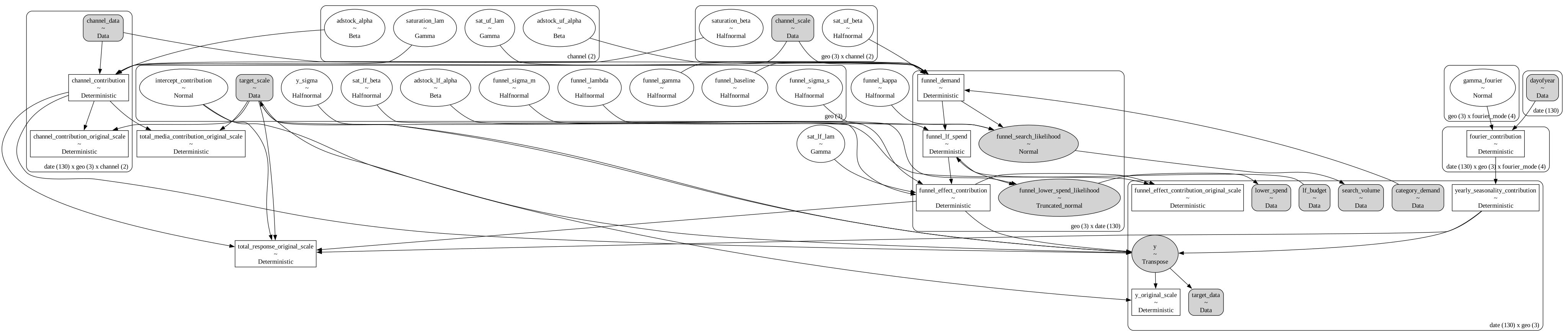
The model graph makes the three likelihoods explicit: the target and the two demand proxies are all children of the same set of latent parameters.
pm.model_to_graphviz(gen.model)
gen.model = do(gen.model, true)

var_names = [
    "y_original_scale",
    "channel_contribution_original_scale",
    "funnel_effect_contribution_original_scale",
    "funnel_demand",
    "funnel_lf_spend",
]
pp_names = ["funnel_lower_spend_likelihood", "funnel_search_likelihood"]

with gen.model:
    idata_gen = pm.sample_prior_predictive(
        draws=1, var_names=var_names + pp_names, random_seed=rng
    )

prior = idata_gen["prior"].sel(chain=0, draw=0)
prior_pp = idata_gen["prior_predictive"].sel(chain=0, draw=0)

y_obs = prior["y_original_scale"].transpose("date", "geo").to_numpy()
demand_true = prior["funnel_demand"].transpose("date", "geo").to_numpy()
lf_spend_true = prior["funnel_lf_spend"].transpose("date", "geo").to_numpy()
lower_spend_obs = (
    prior_pp["funnel_lower_spend_likelihood"].transpose("date", "geo").to_numpy()
)
search_obs = prior_pp["funnel_search_likelihood"].transpose("date", "geo").to_numpy()
direct_true = (
    prior["channel_contribution_original_scale"]
    .transpose("date", "geo", "channel")
    .to_numpy()
)
indirect_raw = (
    prior["funnel_effect_contribution_original_scale"]
    .transpose("date", "geo")
    .to_numpy()
)
/Users/juanitorduz/Documents/pymc-marketing/.venv/lib/python3.14/site-packages/pytensor/link/numba/dispatch/basic.py:234: UserWarning: Numba will use object mode to run truncated_normal_rv{"(),(),(),()->()"}'s perform method. Set `pytensor.config.compiler_verbose = True` to see more details.
  warnings.warn(
Sampling: [funnel_lower_spend_likelihood, funnel_search_likelihood, y]
The true causal decomposition#
The raw funnel_effect_contribution includes the demand that comes from the baseline and the category index, which upper-funnel spend never created. To isolate each channel’s causal indirect contribution we re-run the clamped generative model with that channel’s spend set to zero and subtract. Running the same counterfactual with both channels off lets us measure the non-additivity.
This is the standard mixed-regime construction of mediation analysis: an expectation in which the treatment takes one value in the outcome equation and another in the mediator equation. Mediation Analysis and (In)Direct Effects with PyMC writes those as \(E_{t, t', t''}\) and evaluates them by intervening on the generative model. The cell below does the same, with a clean division of labour: do above clamped the parameters to their true values, and pm.set_data here swaps the inputs. The two “regimes” are a channel’s observed spend and zero spend.
def forward_with_zeroed(channel_mask) -> dict[str, np.ndarray]:
    """Mediated contribution and structural LF spend with masked channels zeroed."""
    media_cf = media_raw.copy()
    media_cf[..., channel_mask] = 0.0
    # The generative model is restored whatever happens in between, so a raise
    # here cannot leave every later truth number on the perturbed media.
    with gen.model:
        try:
            pm.set_data({"channel_data": media_cf})
            idata_cf = pm.sample_prior_predictive(
                draws=1,
                var_names=[
                    "funnel_effect_contribution_original_scale",
                    "funnel_lf_spend",
                ],
                random_seed=rng,
            )
        finally:
            pm.set_data({"channel_data": media_raw})
    draw = idata_cf["prior"].sel(chain=0, draw=0)
    return {
        var: draw[var].transpose("date", "geo").to_numpy()
        for var in ["funnel_effect_contribution_original_scale", "funnel_lf_spend"]
    }


cf_gen = {
    "tv_spend": forward_with_zeroed(np.array([True, False])),
    "social_spend": forward_with_zeroed(np.array([False, True])),
    "both": forward_with_zeroed(np.array([True, True])),
}

indirect_true = np.stack(
    [
        indirect_raw - cf_gen[ch]["funnel_effect_contribution_original_scale"]
        for ch in channels
    ],
    axis=-1,
)
indirect_both = (
    indirect_raw - cf_gen["both"]["funnel_effect_contribution_original_scale"]
)

# The same counterfactual also prices each channel's *induced* lower-funnel spend:
# the structural spend M* with the channel on, minus M* with it off. Because the
# coefficient on D in the M* equation is exactly one, a unit of induced demand is a
# unit of incremental lower-funnel spend; we will need this when defining ROAS.
induced_spend_true = np.stack(
    [lf_spend_true - cf_gen[ch]["funnel_lf_spend"] for ch in channels], axis=-1
)

# Each counterfactual pass restores the generative model's media data itself.
np.testing.assert_allclose(gen.model["channel_data"].get_value(), media_raw)

total_true = direct_true + indirect_true
Sampling: []
Sampling: []
Sampling: []
Note
Unlike the single-channel example, we keep the full date range rather than dropping the first l_max weeks. The generative model and the fitted models apply the same zero-padded adstock, so the early weeks are not an artifact. Dropping them would actually introduce one: the fitted model would be asked to explain weeks whose carryover history had been deleted.
data = xr.Dataset(
    {
        "tv_spend": (("date", "geo"), media_raw[..., 0]),
        "social_spend": (("date", "geo"), media_raw[..., 1]),
        "category_demand": (("date", "geo"), category_demand),
        "lf_budget": (("date", "geo"), lf_budget),
        "lower_spend": (("date", "geo"), lower_spend_obs),
        "search_volume": (("date", "geo"), search_obs),
        "y": (("date", "geo"), y_obs),
        "demand_true": (("date", "geo"), demand_true),
        "lf_spend_true": (("date", "geo"), lf_spend_true),
        "direct_true": (("date", "geo", "channel"), direct_true),
        "indirect_true": (("date", "geo", "channel"), indirect_true),
        "total_true": (("date", "geo", "channel"), total_true),
        "induced_spend_true": (("date", "geo", "channel"), induced_spend_true),
    },
    coords={**coords, "channel": channels},
)

shares = (
    data["indirect_true"].mean("date") / data["total_true"].mean("date")
).to_dataframe(name="indirect share")
shares["indirect share"] = shares["indirect share"].map("{:.1%}".format)
shares
| indirect share | ||
|---|---|---|
| geo | channel | |
| north | tv_spend | 34.9% |
| social_spend | 35.4% | |
| south | tv_spend | 37.7% |
| social_spend | 36.1% | |
| west | tv_spend | 37.2% |
| social_spend | 33.7% |
Between 33.7% and 37.7% (a bit over a third) of every upper-funnel channel’s effect travels through the mediator. Now the non-additivity:
sum_of_singles = float(data["indirect_true"].sum("channel").mean())
joint = float(indirect_both.mean())

pd.DataFrame(
    {
        "sum of single-channel indirect effects": [sum_of_singles],
        "indirect effect of switching both off": [joint],
        "shortfall vs additive": [1 - sum_of_singles / joint],
    },
    index=["mean per week"],
).style.format(
    {
        "sum of single-channel indirect effects": "{:.3f}",
        "indirect effect of switching both off": "{:.3f}",
        "shortfall vs additive": "{:.1%}",
    }
)
| sum of single-channel indirect effects | indirect effect of switching both off | shortfall vs additive | |
|---|---|---|---|
| mean per week | 0.282 | 0.326 | 13.3% |
Because the two channels share one saturating demand pool, per-channel indirect effects computed one at a time understate their joint effect by about 13%. This is not a bug: with a concave response there is no unique way to split a joint effect into per-channel pieces, and leave-one-out attribution is one convention among several. It is worth stating explicitly whenever these numbers inform a budget conversation.
The mediation literature names the leftover rather than rounding it away. Mediation Analysis and (In)Direct Effects with PyMC decomposes a total effect with two mediators as \(\text{TE} = \text{DE} + \text{IIE}_1 + \text{IIE}_2 + \text{INT} + \text{DEP}\). The interaction and dependence terms are precisely the mass the individual indirect effects do not sum to. The axis is different here: our shortfall comes from two treatments pushing on one shared mediator, not from one treatment reaching the outcome through two mediators. But the lesson carries over. The gap is a term with a name, and which convention you report is a choice you owe your reader.
Exploratory visualization#
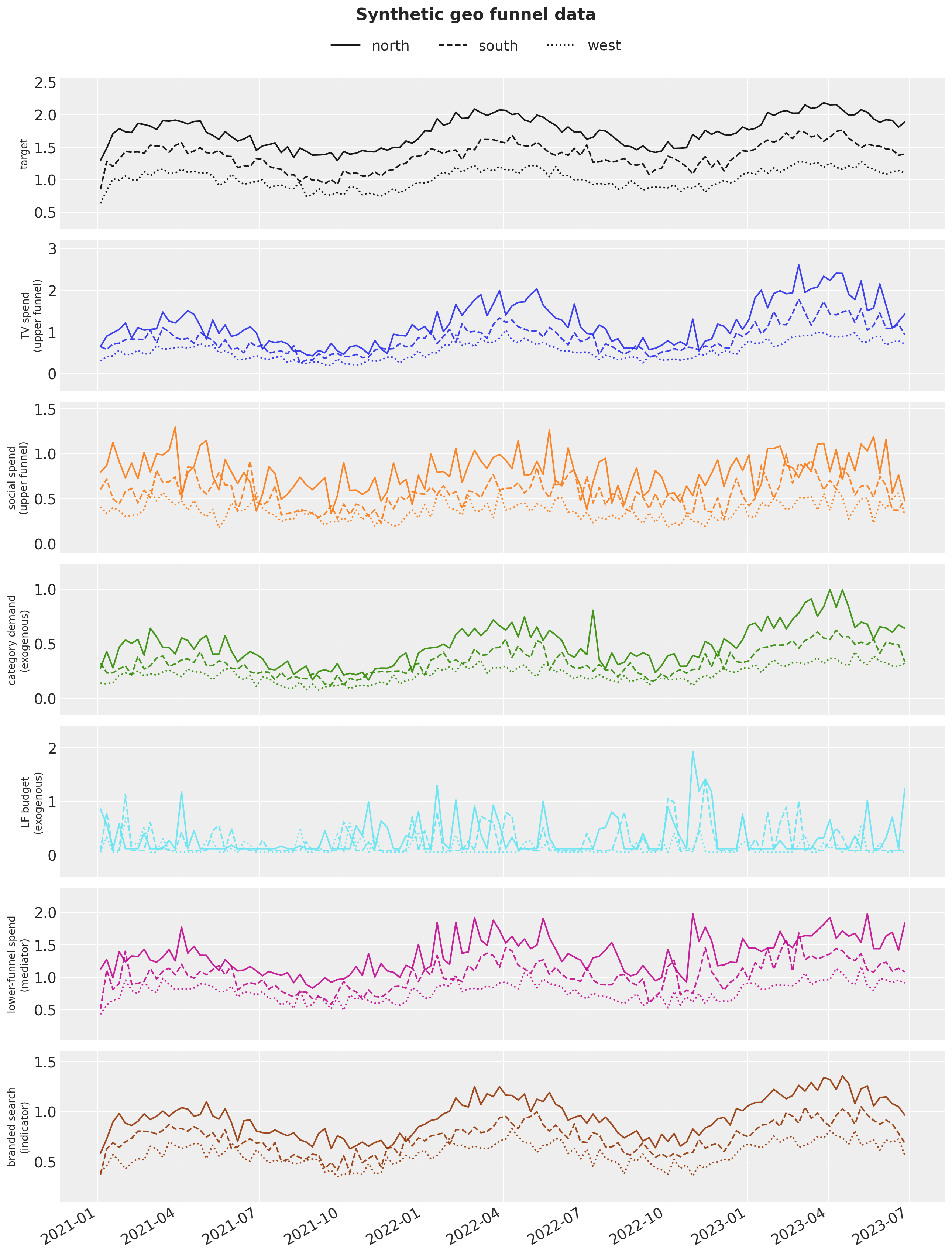
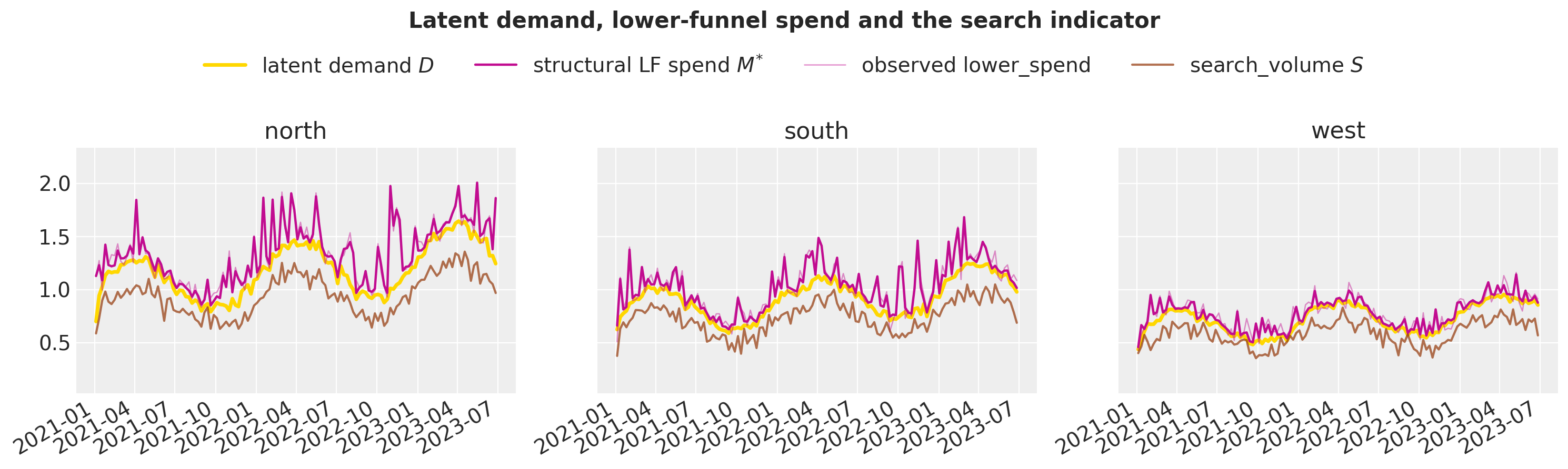
Zooming in on the latent layer shows how the pieces relate. Lower-funnel spend sits above latent demand by the budget-driven wedge \(\lambda_g B_{t,g}\), and the reported series tracks that structural quantity up to reporting noise. Branded search follows demand itself, scaled by \(\kappa\).
What the graph already says#
Before fitting anything, the DAG itself can be interrogated. Each model below is, causally speaking, just a conditioning set: the variables it regresses the target on. Pearl’s backdoor criterion says a set \(Z\) identifies the total effect of a treatment on \(Y\) exactly when two conditions hold: (i) \(Z\) contains no descendant of the treatment, and (ii) \(Z\) d-separates treatment from target in the graph with the treatment’s outgoing edges removed. Both conditions are mechanical graph checks, and networkx ships them. So instead of asserting who is biased and why, we can compute it.
See also
New to backdoor paths and d-separation? Pearl, Glymour and Jewell, Causal Inference in Statistics: A Primer (Wiley, 2016) is the standard gentle introduction to both. The Book of Why (Pearl and Mackenzie, 2018) covers the ideas without the formalism. For how these checks drive model specification in PyMC-Marketing, see the causal identification and causal reasoning and discovery notebooks.
One simplification is worth naming before anything is read off the graph: it is a single time slice. Both adstocks put \(U_{t-k} \to D_t\) and \(M^{*}_{t-k} \to Y_t\) in the data-generating process, and season and t are per-date. Each node here therefore stands for a whole series rather than one week’s value. That is the right reading for an MMM, whose control columns condition on the entire series rather than on row \(t\). But it is a choice the drawing does not show, and a genuinely lagged confounder would need a graph that does.
The same edge list that drew the figure builds the graph:
G = nx.DiGraph([(parent, child) for parent, child, _ in DAG_EDGES])
treatment, outcome = "U1", "Y"

descendants = nx.descendants(G, treatment)

# Backdoor surgery: remove the treatment's outgoing edges.
G_do = G.copy()
G_do.remove_edges_from(list(G.out_edges(treatment)))

# What each model conditions on when estimating tv_spend's effect. Every model
# includes the other channel and the Fourier basis (= the `season` node); they
# differ only in what else they add.
conditioning_sets = {
    "Naive A (mediator as channel)": {"U2", "season", "M"},
    "Naive B (mediator omitted)": {"U2", "season"},
    "Naive B+ (demand as control)": {"U2", "season", "C"},
    "Naive B++ (trend as control)": {"U2", "season", "t"},
    "Naive C (indicator as channel)": {"U2", "season", "S"},
    "(hypothetical: condition on M*)": {"U2", "season", "MS"},
}

rows = {}
for label, Z in conditioning_sets.items():
    forbidden = sorted(Z & descendants)
    blocks = nx.is_d_separator(G_do, {treatment}, {outcome}, Z)
    rows[label] = {
        "conditions on": ", ".join(sorted(Z)),
        "descendant of U₁ in Z": ", ".join(forbidden) or "none",
        "blocks all backdoors": blocks,
        "valid for total effect": blocks and not forbidden,
    }

# The verdicts are symmetric in the treatment: re-run every check with U2 as
# treatment (its conditioning sets swap in the *other* channel, U1).
G_do_u2 = G.copy()
G_do_u2.remove_edges_from(list(G.out_edges("U2")))
descendants_u2 = nx.descendants(G, "U2")
for label, Z in conditioning_sets.items():
    Z_u2 = {("U1" if z == "U2" else z) for z in Z}
    blocks_u2 = nx.is_d_separator(G_do_u2, {"U2"}, {outcome}, Z_u2)
    valid_u2 = blocks_u2 and not (Z_u2 & descendants_u2)
    if (
        blocks_u2 != rows[label]["blocks all backdoors"]
        or valid_u2 != rows[label]["valid for total effect"]
    ):
        raise ValueError(f"verdict differs with U2 as treatment: {label}")

pd.DataFrame(rows).T.style.set_caption(
    f"Backdoor verdicts for treatment {treatment}; "
    f"descendants({treatment}) = {{{', '.join(sorted(descendants))}}}; "
    "every verdict also holds with U2 as the treatment (checked)"
)
| conditions on | descendant of U₁ in Z | blocks all backdoors | valid for total effect | |
|---|---|---|---|---|
| Naive A (mediator as channel) | M, U2, season | M | False | False |
| Naive B (mediator omitted) | U2, season | none | False | False |
| Naive B+ (demand as control) | C, U2, season | none | True | True |
| Naive B++ (trend as control) | U2, season, t | none | False | False |
| Naive C (indicator as channel) | S, U2, season | S | False | False |
| (hypothetical: condition on M*) | MS, U2, season | MS | True | False |
A verdict is a boolean, and a boolean cannot say how a set fails or what it leaves behind. Counting the backdoor paths each conditioning set leaves open can, so a short helper does exactly that. Every count it produces is cross-checked against nx.is_d_separator, so the hand-rolled logic cannot drift from the library’s verdicts.
Tip
Conditioning on a collider opens paths that something else must close again. The last row below (Naive B+ without its Fourier basis) shows the effect at C: it is the seasonal basis that does the closing there.
backdoor_paths = list(nx.all_simple_paths(G_do.to_undirected(), treatment, outcome))


def open_paths(Z):
    """Backdoor paths that conditioning set ``Z`` leaves open."""
    left_open = []
    for path in backdoor_paths:
        blocked = False
        for before, node, after in zip(path, path[1:], path[2:], strict=False):
            if G_do.has_edge(before, node) and G_do.has_edge(after, node):
                # A collider blocks unless it, or a descendant, is in Z.
                blocked = not ({node} | nx.descendants(G_do, node)) & Z
            else:
                blocked = node in Z
            if blocked:
                break
        if not blocked:
            left_open.append(path)
    return left_open


def render(path):
    """``U1 <- N -> C -> D -> MS -> Y``: arrows point the way the graph does."""
    out = [path[0]]
    for before, node in itertools.pairwise(path):
        out += ["->" if G_do.has_edge(before, node) else "<-", node]
    return " ".join(out)


adjustment_sets = {
    "the seasonal basis alone": {"season"},
    "Naive B": {"U2", "season"},
    "Naive B+": {"U2", "season", "C"},
    "Naive B++": {"U2", "season", "t"},
    "Naive B+ without the Fourier basis": {"U2", "C"},
}

# Certify the helper against the library: a set leaves zero paths open exactly
# when `is_d_separator` says it blocks them all.
for Z in adjustment_sets.values():
    if (len(open_paths(Z)) == 0) != nx.is_d_separator(G_do, {treatment}, {outcome}, Z):
        raise ValueError(f"open_paths disagrees with is_d_separator for {sorted(Z)}")

pd.DataFrame(
    {
        "conditioning set": {
            label: "{" + ", ".join(sorted(Z)) + "}"
            for label, Z in adjustment_sets.items()
        },
        "open backdoor paths": {
            label: len(open_paths(Z)) for label, Z in adjustment_sets.items()
        },
    }
).style.set_caption(
    f"Of {len(backdoor_paths)} backdoor paths from {treatment} to {outcome}"
)
| conditioning set | open backdoor paths | |
|---|---|---|
| the seasonal basis alone | {season} | 6 |
| Naive B | {U2, season} | 4 |
| Naive B+ | {C, U2, season} | 0 |
| Naive B++ | {U2, season, t} | 1 |
| Naive B+ without the Fourier basis | {C, U2} | 9 |
pd.DataFrame(
    [
        {"conditioning set": label, "open path": render(path)}
        for label, Z in adjustment_sets.items()
        if 1 <= len(open_paths(Z)) <= 4
        for path in open_paths(Z)
    ]
).set_index("conditioning set")
| open path | |
|---|---|
| conditioning set | |
| Naive B | U1 <- t -> U2 <- N -> C -> D -> MS -> Y |
| Naive B | U1 <- t -> C -> D -> MS -> Y |
| Naive B | U1 <- N -> U2 <- t -> C -> D -> MS -> Y |
| Naive B | U1 <- N -> C -> D -> MS -> Y |
| Naive B++ | U1 <- N -> C -> D -> MS -> Y |
Reading the verdicts off the table:
Naive B fails condition (ii). With only the other channel and the seasonal basis conditioned, the backdoor \(U_1 \leftarrow t \to C \to D \to M^{*} \to Y\) stays open. So does its twin through the drivers’ shared noise, \(U_1 \leftarrow N \to C \to D \to M^{*} \to Y\). Note what this is not: omitting the mediator is the correct move for a total effect. That is what makes it a total effect. The graph-level defect is the open backdoor through the shared driver. Its trend strand is the co-movement the residual-correlation table showed surviving the seasonal adjustment on the TV side.
Naive B+ is valid; Naive B++ is not. Both fork nodes, \(t\) and \(N\), sit upstream of both the treatment and \(C\), and \(C\) sits on both paths downstream of them. Conditioning on the observed category index therefore blocks the trend strand and the noise strand at once. Conditioning on \(t\) blocks only the strand it names. The noise path stays open, and \(N\) is unobservable, so
Naive B++cannot close it by adding a column. Neither variable is a descendant of the treatment, so what separates them is coverage, not condition (i).The path count above says the same thing more concretely. Of the 43 backdoor paths,
Naive Bleaves four open,Naive B++exactly one (the noise fork, listed above), andNaive B+none.Naive B’s four have one structure: two are the forks themselves, and two are hybrids that enter on one fork and exit on the other, spliced at the other channel.season, \(t\) and \(N\) all point into \(U_2\), so the other channel is a collider as well as a regressor. Conditioning on it closes the paths that run through it and opens the ones that meet at it. The first row measures exactly that: the seasonal basis alone leaves six paths open, and adding \(U_2\) leaves four. All four exit through \(C \to D \to M^{*} \to Y\), which is why conditioning on \(C\) closes every one of them andNaive B+scores valid.Naive B+’s credential is joint with the Fourier basis. \(C\) is a collider too:season, \(t\) and \(N\) point into it exactly as they do into \(U_2\). Conditioning on it therefore opens every path that meets there, and it is the seasonal basis (present in every model) that closes them again. Take the basis away and the same conditioning set leaves nine paths open, as the last row shows. A reader who switchesyearly_seasonalityoff does not get a slightly worseNaive B+; they get a specification with no credential at all.Naive A and Naive C fail condition (i): each conditions on a descendant of the treatment (
Mvia \(U_1 \to D \to M^{*} \to M\);Svia \(U_1 \to D \to S\)), cutting into the causal path itself. No amount of extra controls repairs that. (Descendants of \(D\) also open collider paths at \(D\). On this graph every such path is re-blocked at \(U_2\), which both conditioning sets contain, but free-by-accident is a property of this graph, not of the move.)The hypothetical last row is the interesting one. Conditioning on the structural \(M^{*}\) would block every backdoor, yet it is still invalid for the total effect, for exactly the same reason: it is a descendant, and conditioning on it is what defines the direct effect instead.
That last distinction can be made precise. Removing the direct edge \(U_1 \to Y\) and asking whether the conditioning set separates treatment from target tests whether it isolates the direct path:
G_direct = G.copy()
G_direct.remove_edge(treatment, "Y")

pd.DataFrame(
    {
        "isolates the direct effect": {
            "M* (structural)": nx.is_d_separator(
                G_direct, {treatment}, {outcome}, {"U2", "season", "MS"}
            ),
            "M (noisy observation, what Naive A has)": nx.is_d_separator(
                G_direct, {treatment}, {outcome}, {"U2", "season", "M"}
            ),
        }
    }
)
| isolates the direct effect | |
|---|---|
| M* (structural) | True |
| M (noisy observation, what Naive A has) | False |
So Naive A is not estimating the total effect badly; it is (approximately) estimating the direct effect. Approximately, because it conditions on the noisy observation M rather than the structural M*. Strict d-separation fails through the measurement noise, and the approximation is good exactly to the extent \(\sigma^M\) is small. Keep this in mind for the comparisons below, where we benchmark Naive A against the quantity it actually answers for.
Finally, the graph can be asked what adjustment it would recommend:
# Sorted: a set's repr order is not stable across processes, and these outputs
# are meant to reproduce exactly.
unrestricted = sorted(nx.find_minimal_d_separator(G_do, {treatment}, {outcome}))

# `N` is deliberately absent from `observable`: no dataset carries the drivers'
# shared noise. A practitioner can only act on the restricted answer.
observable = {"U2", "season", "C", "B", "M", "S", "t"} - descendants
restricted = sorted(
    nx.find_minimal_d_separator(
        G_do,
        {treatment},
        {outcome},
        included={"U2", "season"},
        restricted=observable | {"U2", "season"},
    )
)

pd.DataFrame(
    {
        "a minimal separator": {
            "unrestricted": str(unrestricted),
            "observables only": str(restricted),
        }
    }
)
| a minimal separator | |
|---|---|
| unrestricted | ['N', 'season', 't'] |
| observables only | ['C', 'U2', 'season'] |
# `find_minimal_d_separator` returns *a* minimal separator, not *the* minimal
# one. On a graph this size the whole lattice is enumerable (2**10 subsets),
# so count them all with `nx.is_minimal_d_separator` instead of over-reading
# one answer.
def minimal_separators(candidates):
    """Every minimal d-separator of (treatment, outcome) drawn from ``candidates``."""
    return sorted(
        [
            sorted(Z)
            for size in range(len(candidates) + 1)
            for Z in itertools.combinations(sorted(candidates), size)
            if nx.is_minimal_d_separator(G_do, {treatment}, {outcome}, set(Z))
        ],
        key=lambda Z: (len(Z), Z),
    )


pd.DataFrame(
    [
        {"restriction": "unrestricted", "minimal separator": str(Z)}
        for Z in minimal_separators(set(G) - {treatment, outcome})
    ]
    + [
        {"restriction": "observables only", "minimal separator": str(Z)}
        for Z in minimal_separators(observable | {"U2", "season"})
    ]
).set_index("restriction")
| minimal separator | |
|---|---|
| restriction | |
| unrestricted | ['C', 'U2', 'season'] |
| unrestricted | ['D', 'U2', 'season'] |
| unrestricted | ['MS', 'U2', 'season'] |
| unrestricted | ['N', 'season', 't'] |
| observables only | ['C', 'U2', 'season'] |
Unrestricted, one minimal separator the graph names is the season, the trend and \(N\), which no dataset contains. Read that as a tie-break rather than an obstacle. The enumeration finds four minimal separators, and \(\{C, U_2, \text{season}\}\) is one of them, exactly as small. find_minimal_d_separator returns whichever branch it walks into, so the latent variable in its answer is not the graph refusing to be adjusted. Minimality is not the only filter, though. The other two, \(\{D, U_2, \text{season}\}\) and \(\{M^{*}, U_2, \text{season}\}\), are ruled out a second time over by condition (i): both \(D\) and \(M^{*}\) are descendants of the treatment, as the verdict table’s caption records. Unobservable, or a descendant, or the one usable alternative: that is the whole lattice.
Restricted to observed, non-descendant variables, with the other channel and the seasonal basis already in every model, the answer is \(\{C, U_2, \text{season}\}\). Now the enumeration says it is the only minimal one, with \(U_2\) load-bearing: the same \(U_2\) whose collider opens two paths in the count above. Load-bearing and collider-opening at once is not a contradiction; it is why a separation test and a path count answer different questions. The graph nominates Naive B+’s specification, and it drops \(t\) altogether, because conditioning on the observed category index blocks the trend strand and the noise strand in one move.
Note
With networkx unpinned, a library upgrade could legitimately change one thing in this section: the order in which the open-path listing and the find_minimal_d_separator branch are returned. Every count and every verdict is immune.
Naive B++ is the cheaper specification: a column computed from the calendar, no extra data series. But it is valid only conditionally. It closes the trend fork and leaves the noise fork open. Reading it as a valid total-effect estimator is therefore an assumption about the size of the driver-noise correlation we measured above: \(|r| \le 0.18\) per geo against a floor of 0.13, and \(\le 0.13\) pooled against 0.11. That is the honest status of most trend controls in practice, and it is worth stating as an assumption rather than a verdict. Both models are fit below, so the graph’s ranking can be checked against the truth rather than taken on faith. The empirical result is not the one the ranking suggests, which is the point of checking. The six verdicts in the table also hold with U2 as the treatment, recomputed cell by cell in the loop that built it rather than assumed; the direct-effect and separator checks are stated for U1 only.
One model is deliberately missing from this analysis: the funnel model is not identified by an adjustment set at all. It identifies by specifying the full structural system, and that buys correctness exactly insofar as the demand equation is correctly specified (including \(C\)’s role in it) and nothing unobserved confounds \(M^{*} \to Y\). The backdoor machinery cannot certify those assumptions; the parameter-recovery and proxy-predictive checks later in the notebook are their empirical substitute.
One more thing the graph makes testable. The exclusion restriction “the budget enters lower-funnel spend but not branded search” implies \(B \perp S\) marginally. Their only connecting path runs through the collider at \(M^{*}\), which stays blocked as long as nothing downstream of it is conditioned on:
pd.DataFrame(
    {
        "B ⊥ S given Z": {
            "Z = {}": nx.is_d_separator(G, {"B"}, {"S"}, set()),
            "Z = {Y}": nx.is_d_separator(G, {"B"}, {"S"}, {"Y"}),
            "Z = {M}": nx.is_d_separator(G, {"B"}, {"S"}, {"M"}),
        }
    }
)
| B ⊥ S given Z | |
|---|---|
| Z = {} | True |
| Z = {Y} | False |
| Z = {M} | False |
pd.DataFrame(
    {
        "corr(lf_budget, search_volume)": {
            geo: np.corrcoef(lf_budget[:, gi], search_obs[:, gi])[0, 1]
            for gi, geo in enumerate(geos)
        }
    }
).style.format("{:+.3f}")
| corr(lf_budget, search_volume) | |
|---|---|
| north | -0.053 |
| south | +0.019 |
| west | -0.218 |
Two of the three per-geo correlations sit at zero, as the graph says they should. west’s -0.218 does not. It runs about two and a half times the sampling standard error quoted above, the kind of tail a marginal-independence check throws up now and again on 130 weeks. The restriction is exact in the DGP, so this is a statement about the draw rather than about the graph, and \(\lambda\) is still cleanly recovered below. It is worth printing rather than hiding: on real data this is exactly the ambiguity you would have to resolve. Two caveats about running the check. It only works per geo: pooled across regions, both series scale with market size, and that common cause manufactures a spurious positive correlation. And it only works on the raw series: conditioning on anything downstream of \(M^{*}\), including the target, opens the collider. If real data failed this check systematically, the exclusion restriction, and with it the identification of \(\lambda\), would be suspect before a single model was fit.
Note
For production use, CausalGraphModel automates adjustment-set selection from a DAG string. Its recommendation is coarser than the checks above. We ran the checks with raw networkx so that the reasoning stays visible.
Fitting the models#
We now fit the six model structures defined at the top of the notebook, all on the same synthetic data. The five naive models differ from one another only in which observed series they condition on, so differences among them are structural.
The funnel model additionally observes more than any of them: two extra likelihood series (lower_spend, search_volume) and two extra inputs (category_demand, lf_budget). Where it has an advantage, that advantage comes from structure and information together, a distinction worth keeping in mind when reading the comparisons.
frame = (
    data[
        [
            "tv_spend",
            "social_spend",
            "lower_spend",
            "search_volume",
            "category_demand",
            "y",
        ]
    ]
    .to_dataframe()
    .reset_index()
)

X_upper = frame[["date", "geo", *channels]]
X_with_mediator = frame[["date", "geo", *channels, "lower_spend"]]
X_with_search = frame[["date", "geo", *channels, "search_volume"]]
X_with_control = frame[["date", "geo", *channels, "category_demand"]]
# The growth trend as a control regressor: observable from the calendar alone.
frame["t"] = frame["date"].map(dict(zip(date_range, t, strict=True)))
X_with_trend = frame[["date", "geo", *channels, "t"]]
y = frame["y"]

sample_kwargs = dict(chains=4, tune=1_000, draws=1_000, target_accept=0.95)
sampler_config = {"nuts_sampler": "nutpie"}
Naive A (mediator as channel): the mediator as an ordinary channel#
This is what most production MMMs do when they have upper- and lower-funnel spend in the same table: list them side by side. It is not an unreasonable model. In this DAG lower-funnel spend really does drive the target, so the coefficient it estimates is a real thing. But as the d-separation table showed, conditioning on the mediator blocks the indirect path. The upper channels are credited with at most their direct effect, and the lower-funnel channel keeps the credit for demand they created. Naive A (mediator as channel) is not a broken model so much as a model that silently answers a different question, the direct effect. We will benchmark it against that quantity as well as against the total.
naive_a = make_mmm([*channels, "lower_spend"], sampler_config=sampler_config)
naive_a.build_model(X_with_mediator, y)
naive_a.add_original_scale_contribution_variable(var=["channel_contribution", "y"])
naive_a.fit(X_with_mediator, y, random_seed=rng, **sample_kwargs)
naive_a.sample_posterior_predictive(X_with_mediator, random_seed=rng);
NUTS[nutpie]: [y_sigma, gamma_fourier, adstock_alpha, saturation_lam, saturation_beta, intercept_contribution]
Sampling: [y]
Naive B (mediator omitted)#
Here the two upper channels are the only media. Causally this is the right estimand: not conditioning on the mediator is exactly what makes a total effect a total effect. Naive B (mediator omitted) has two distinct problems, and they will land on different channels. The first is the one the graph isolated: the open backdoor through the shared growth trend, which the residual-correlation table showed is material for TV and absent for social. The second the graph is silent about. With the mediator omitted, each response curve also has to absorb the demand its channel creates downstream, mediated through a saturating pool the model does not represent. Where each part lands, we will let the results say.
naive_b = make_mmm(channels, sampler_config=sampler_config)
naive_b.build_model(X_upper, y)
naive_b.add_original_scale_contribution_variable(var=["channel_contribution", "y"])
naive_b.fit(X_upper, y, random_seed=rng, **sample_kwargs)
naive_b.sample_posterior_predictive(X_upper, random_seed=rng);
NUTS[nutpie]: [y_sigma, gamma_fourier, adstock_alpha, saturation_lam, saturation_beta, intercept_contribution]
Sampling: [y]
Naive B+ (demand as control): mediator omitted, category demand as a control#
This is the adjustment the d-separation analysis nominated: block the remaining backdoors with the observed category index, which sits downstream of both forks in the shared driver. MMM takes it as an ordinary control column (a linear term with a per-geo coefficient, no adstock or saturation), which is one argument and no new machinery:
naive_bplus = make_mmm(
    channels, control_columns=["category_demand"], sampler_config=sampler_config
)
naive_bplus.build_model(X_with_control, y)
naive_bplus.add_original_scale_contribution_variable(var=["channel_contribution", "y"])
naive_bplus.fit(X_with_control, y, random_seed=rng, **sample_kwargs)
naive_bplus.sample_posterior_predictive(X_with_control, random_seed=rng);
NUTS[nutpie]: [y_sigma, gamma_fourier, gamma_control, adstock_alpha, saturation_lam, saturation_beta, intercept_contribution]
Sampling: [y]
Two things to note before seeing results. First, on the graph this is a formally valid total-effect estimator at the cost of one extra column. If all you need is total ROAS per upper channel, specifications like this are the honest baseline the funnel model has to beat. Second, its control is a linear stand-in for a path that is truly nonlinear: \(C\) enters through the demand equation and then a saturating conversion. Some residual bias is therefore possible even though the graph verdict is clean, because d-separation is about which variables suffice, not about functional form. Keep that caveat in mind: it returns with force below.
Naive B++ (trend as control): mediator omitted, the trend as a control#
The second candidate is the cheapest specification available here: no extra data series at all, since the regressor is a function of the calendar. On the graph it is valid only under the extra assumption that the drivers’ shared noise is negligible. That is the kind of assumption trend controls usually rest on, and we sized it above rather than waved at it. The same functional-form caveat applies as for Naive B+ (demand as control): the trend reaches the target through softplus-rectified plans and a saturating conversion, and a linear term stands in for all of it.
naive_bpp = make_mmm(channels, control_columns=["t"], sampler_config=sampler_config)
naive_bpp.build_model(X_with_trend, y)
naive_bpp.add_original_scale_contribution_variable(var=["channel_contribution", "y"])
naive_bpp.fit(X_with_trend, y, random_seed=rng, **sample_kwargs)
naive_bpp.sample_posterior_predictive(X_with_trend, random_seed=rng);
NUTS[nutpie]: [y_sigma, gamma_fourier, gamma_control, adstock_alpha, saturation_lam, saturation_beta, intercept_contribution]
Sampling: [y]
Naive C (indicator as channel): the indicator as a channel#
Branded search volume is the most tempting variable in the whole dataset. It correlates beautifully with sales, it is free, and it arrives weekly. So it ends up in the channel list.
It causes nothing. Because it is a descendant of latent demand, conditioning on it blocks \(U \to D \to M^{*} \to Y\) just as surely as conditioning on the mediator itself would. This is textbook post-treatment conditioning, on a variable that has no causal role at all.
naive_c = make_mmm([*channels, "search_volume"], sampler_config=sampler_config)
naive_c.build_model(X_with_search, y)
naive_c.add_original_scale_contribution_variable(var=["channel_contribution", "y"])
naive_c.fit(X_with_search, y, random_seed=rng, **sample_kwargs)
naive_c.sample_posterior_predictive(X_with_search, random_seed=rng);
NUTS[nutpie]: [y_sigma, gamma_fourier, adstock_alpha, saturation_lam, saturation_beta, intercept_contribution]
Sampling: [y]
The funnel model#
The funnel model has the two upper channels (their direct effects) plus the FunnelEffect, which reads the mediator data from the Dataset and fits the target and both proxies jointly. Note the plumbing discussed earlier: we build from the Dataset and fit with the long frame.
ds_fit = make_dataset(
    media_raw, lower_spend_obs, search_obs, category_demand, lf_budget
)
y_fit = xr.DataArray(y_obs, dims=("date", "geo"), coords=coords)

funnel = make_mmm(channels, sampler_config=sampler_config)
funnel.add_mu_effect(make_funnel_effect())
funnel.build_model(X=ds_fit, y=y_fit)
funnel.add_original_scale_contribution_variable(
    var=["channel_contribution", "funnel_effect_contribution", "y"]
)
funnel.fit(X=X_upper, y=y, random_seed=rng, **sample_kwargs)
funnel.sample_posterior_predictive(X_upper, random_seed=rng);
NUTS[nutpie]: [y_sigma, adstock_lf_alpha, funnel_lambda, adstock_uf_alpha, sat_uf_lam, sat_uf_beta, funnel_gamma, funnel_baseline, sat_lf_lam, sat_lf_beta, gamma_fourier, adstock_alpha, saturation_lam, saturation_beta, intercept_contribution, funnel_sigma_s, funnel_kappa, funnel_sigma_m]
/Users/juanitorduz/Documents/pymc-marketing/.venv/lib/python3.14/site-packages/pytensor/link/numba/dispatch/basic.py:234: UserWarning: Numba will use object mode to run truncated_normal_rv{"(),(),(),()->()"}'s perform method. Set `pytensor.config.compiler_verbose = True` to see more details.
  warnings.warn(
Sampling: [funnel_lower_spend_likelihood, funnel_search_likelihood, y]
Diagnostics#
models = {
    "Naive A": naive_a,
    "Naive B": naive_b,
    "Naive B+": naive_bplus,
    "Naive B++": naive_bpp,
    "Naive C": naive_c,
    "Funnel": funnel,
}

# Scalar parameters only: summarising the date x geo deterministics would
# dominate this cell's runtime.
scalar_params = [
    "intercept_contribution",
    "adstock_alpha",
    "saturation_lam",
    "saturation_beta",
    "gamma_fourier",
    "gamma_control",
    "y_sigma",
    "funnel_baseline",
    "funnel_gamma",
    "funnel_lambda",
    "funnel_kappa",
    "funnel_sigma_m",
    "funnel_sigma_s",
    "adstock_uf_alpha",
    "sat_uf_lam",
    "sat_uf_beta",
    "adstock_lf_alpha",
    "sat_lf_lam",
    "sat_lf_beta",
]

sampler_diagnostics = {}
for label, model in models.items():
    present = [v for v in scalar_params if v in model.idata.posterior]
    sampler_diagnostics[label] = {
        "divergences": int(model.idata["sample_stats"]["diverging"].sum()),
        "max r-hat": float(az.summary(model.idata, var_names=present)["r_hat"].max()),
    }

pd.DataFrame(sampler_diagnostics).T.style.format({"max r-hat": "{:.3f}"})
| divergences | max r-hat | |
|---|---|---|
| Naive A | 0.000000 | 1.010 |
| Naive B | 0.000000 | 1.010 |
| Naive B+ | 0.000000 | 1.010 |
| Naive B++ | 0.000000 | 1.010 |
| Naive C | 0.000000 | 1.000 |
| Funnel | 0.000000 | 1.000 |
Posterior predictive checks#
The funnel model has three observed quantities. All of them should be well recovered.
funnel.plot_suite = "new"

pc = funnel.plot.diagnostics.posterior_predictive(
    hdi_prob=0.94, return_as_pc=True, figsize=(13, 8)
)
fig = pc.viz["figure"].item()

for i, geo in enumerate(geos):
    ax = pc.viz["plot"].sel(geo=geo).item()
    ax.set_xlabel("date" if i == len(geos) - 1 else "")
    ax.set_ylabel("")
    ax.set_title(geo)

fig.supylabel("target")
fig.suptitle(
    "Funnel model: target posterior predictive", fontsize=14, fontweight="bold"
)
fig.autofmt_xdate()
fig.set_layout_engine("tight", rect=(0.01, 0, 1, 0.97))
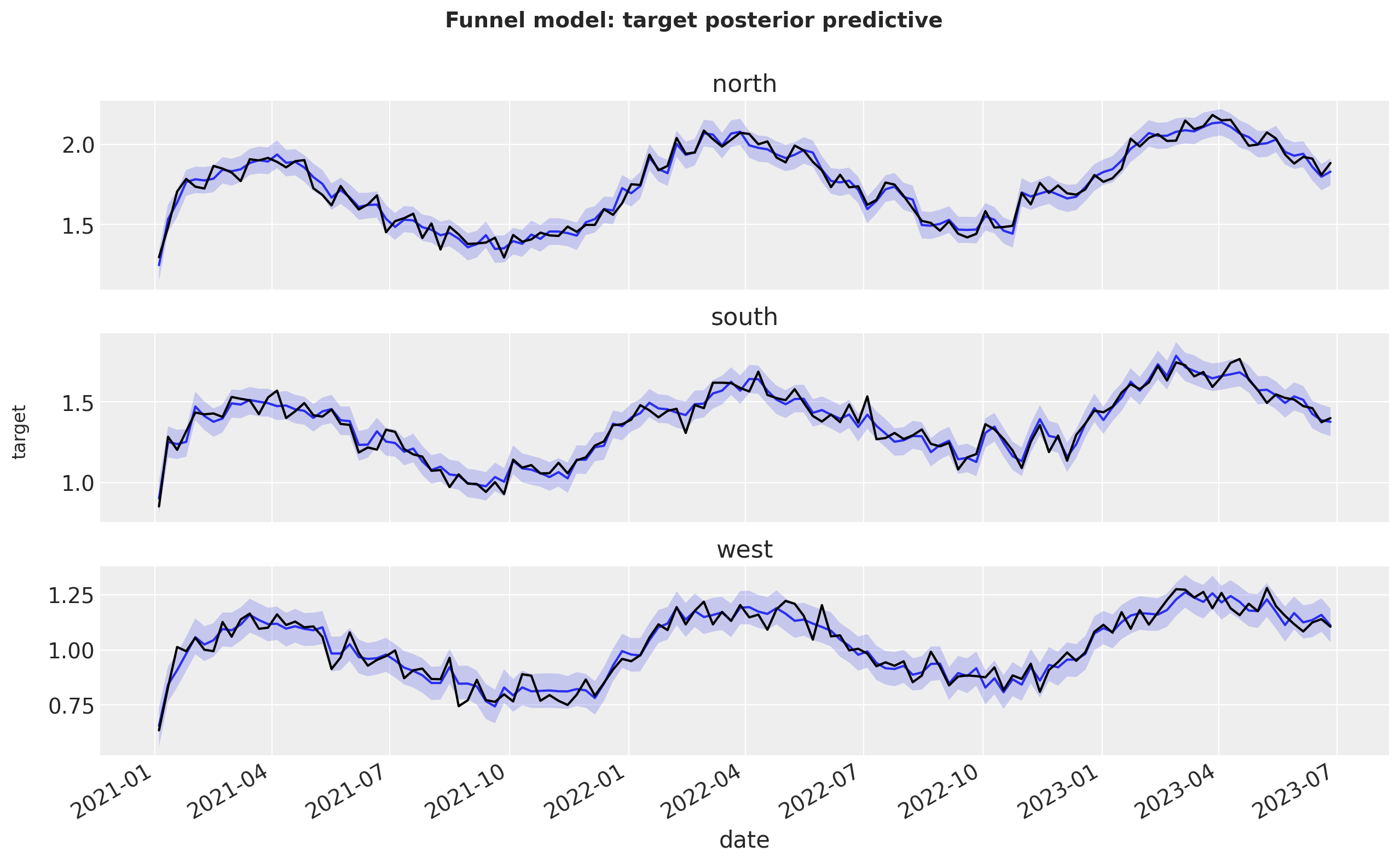
The other two are the effect’s own likelihoods, which have no built-in plot, so we draw them by hand.
Those panels quote a posterior HDI, as does nearly every figure from here on, so a small helper for the interval bounds comes first:
def hdi_bounds(da, prob: float = 0.94):
    """Return (lower, upper) HDI DataArrays for a posterior DataArray."""
    h = az.hdi(da, prob=prob)
    if isinstance(h, xr.Dataset):
        h = h[next(iter(h.data_vars))]
    return h.sel(ci_bound="lower"), h.sel(ci_bound="upper")
proxies = [
    ("funnel_lower_spend_likelihood", "lower_spend", "Lower-funnel spend", "C3"),
    ("funnel_search_likelihood", "search_volume", "Branded search volume", "C4"),
]

fig, axes = plt.subplots(
    nrows=len(proxies), ncols=len(geos), figsize=(15, 8), sharex=True
)
for row, (var, observed, title, color) in enumerate(proxies):
    pp = funnel.idata.posterior_predictive[var]
    lo, hi = hdi_bounds(pp)
    mean = pp.mean(dim=["chain", "draw"])
    for col, geo in enumerate(geos):
        ax = axes[row, col]
        ax.fill_between(
            date_range, lo.sel(geo=geo), hi.sel(geo=geo), alpha=0.3, color=color
        )
        ax.plot(date_range, mean.sel(geo=geo), color=color, label="posterior mean")
        ax.plot(
            date_range,
            data[observed].sel(geo=geo),
            color="black",
            alpha=0.7,
            label="observed",
        )
        ax.set(title=f"{title}, {geo}")
axes[0, 0].legend(loc="upper left")
fig.suptitle(
    "Funnel model: demand-proxy posterior predictives",
    fontsize=15,
    fontweight="bold",
)
fig.autofmt_xdate()
fig.set_layout_engine("tight")
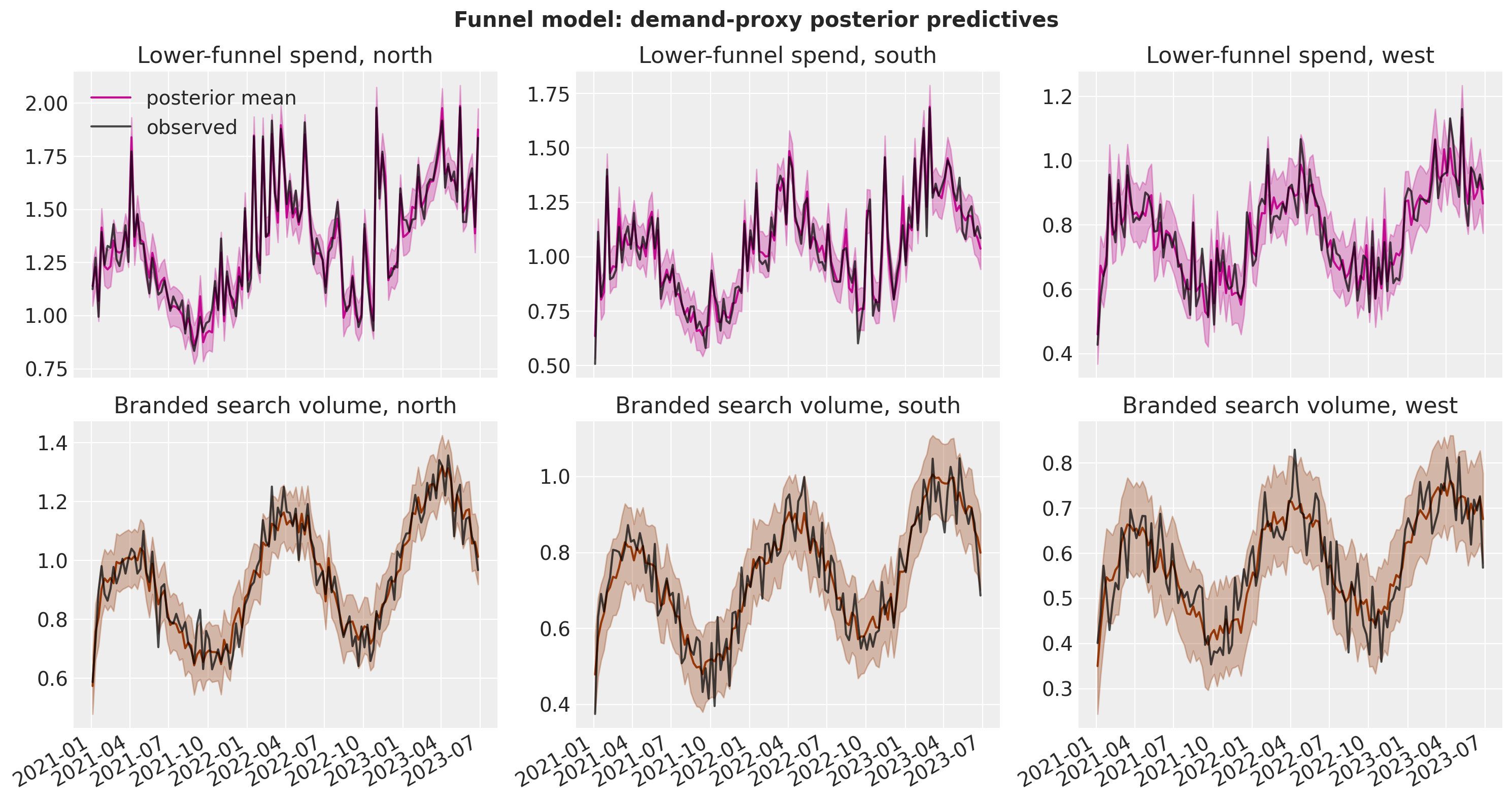
Parameter recovery#
Important
Where this lands. The funnel model recovers the ground truth, but the direct and demand paths are only weakly identified apart: in all six channel-geo cells the two amplitudes miss in opposite directions. That seesaw is a property of two paths originating at the same spend, not six independent misses, and the total effects further down survive it. west is the hardest geo, by construction.
Because we generated the data we can check the funnel model against the truth. One subtlety carries over from the basic notebook and gets slightly more involved here. The MMM fits on an internally scaled target, so every parameter that acts on the scale of the target mean (the intercept, the two saturation amplitudes and the Fourier coefficients) must be multiplied by target_scale before comparing with the ground truth. With dims=() scaling that factor is per geo, and xarray applies it by label for us. Parameters acting on the inputs (adstock decays, saturation curvatures) or on the mediator scale (everything in the demand equation) are scale-free and compare directly.
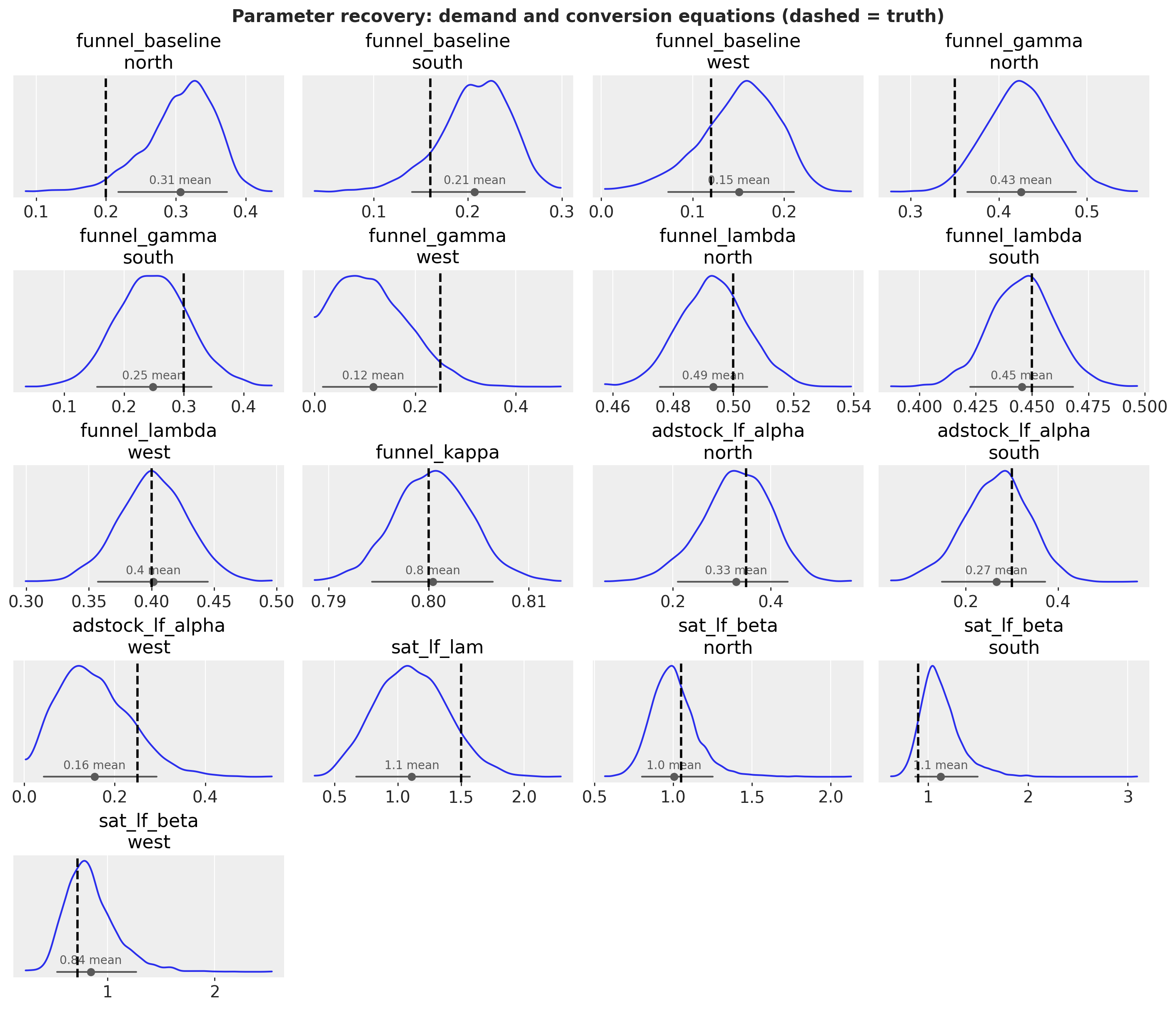
The two loadings that carry the new structure, funnel_lambda and funnel_kappa, are pinned down tightly, which is what we want. They decide how much of lower-funnel spend is demand-driven and how strongly branded search tracks demand. Not everything in the new block is that sharp: the recovery table below puts adstock_lf_alpha in west at 0.156 against a true 0.250, covered but loose.
It is worth checking that \(\lambda\) is genuinely identified rather than simply returning its prior: an unidentified parameter still produces a posterior that happily brackets the truth. Two things to look at: how much the data sharpened it relative to the prior, and whether it traded off against the demand baseline it shares a level with.
prior_lambda_sd = 0.5 * np.sqrt(1 - 2 / np.pi)  # sd of HalfNormal(sigma=0.5)
lambda_draws = funnel.idata.posterior["funnel_lambda"]

identification = pd.DataFrame(
    {
        "posterior mean": lambda_draws.mean(dim=["chain", "draw"]).to_series(),
        "true": pd.Series(true["funnel_lambda"], index=geos),
        "posterior sd / prior sd": (
            lambda_draws.std(dim=["chain", "draw"]) / prior_lambda_sd
        ).to_series(),
        "corr(lambda, baseline)": pd.Series(
            {
                geo: float(
                    xr.corr(
                        lambda_draws.sel(geo=geo),
                        funnel.idata.posterior["funnel_baseline"].sel(geo=geo),
                    )
                )
                for geo in geos
            }
        ),
    }
)
identification.style.format("{:.3f}")
| posterior mean | true | posterior sd / prior sd | corr(lambda, baseline) | |
|---|---|---|---|---|
| north | 0.493 | 0.500 | 0.037 | -0.100 |
| south | 0.445 | 0.450 | 0.048 | 0.036 |
| west | 0.401 | 0.400 | 0.091 | -0.061 |
The data shrinks \(\lambda\) to a small fraction of its prior width, and its correlation with the demand baseline is close to zero. That is the exclusion restriction doing its job: the budget enters lower-funnel spend but not branded search, so the search equation pins the baseline while the budget’s promotional spikes pin \(\lambda\). Had we generated a flat, always-on budget instead, these two would have been hopelessly confounded and no amount of sampling would have helped.
Now the media parameters:
recovery_plot(
    [
        "adstock_uf_alpha",
        "sat_uf_lam",
        "sat_uf_beta",
        "adstock_alpha",
        "saturation_lam",
        "saturation_beta",
    ],
    "Parameter recovery: media transformations (dashed = truth)",
    (14, 14),
);
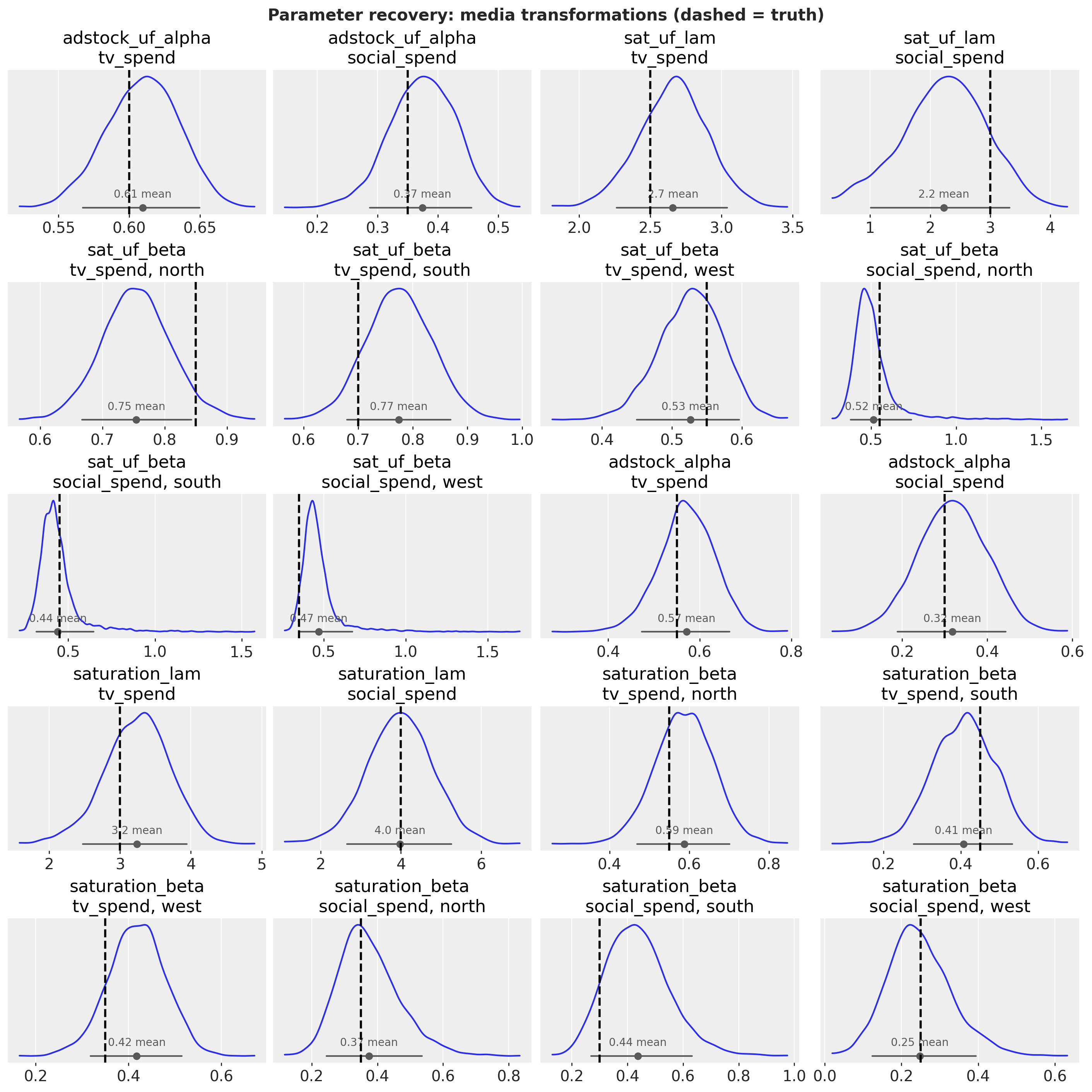
Thirty-seven KDE panels across two figures are good for shapes and bad for checking claims. So here is the same information as numbers for every one of them: posterior mean, 94% HDI, truth, and whether the interval covers it:
| mean | hdi 3% | hdi 97% | true | covered | ||
|---|---|---|---|---|---|---|
| parameter | cell | |||||
| funnel_baseline | north | 0.307 | 0.208 | 0.387 | 0.200 | False |
| south | 0.207 | 0.135 | 0.275 | 0.160 | True | |
| west | 0.150 | 0.067 | 0.225 | 0.120 | True | |
| funnel_gamma | north | 0.425 | 0.356 | 0.500 | 0.350 | False |
| south | 0.249 | 0.141 | 0.365 | 0.300 | True | |
| west | 0.117 | 0.002 | 0.240 | 0.250 | False | |
| funnel_lambda | north | 0.493 | 0.473 | 0.516 | 0.500 | True |
| south | 0.445 | 0.417 | 0.472 | 0.450 | True | |
| west | 0.401 | 0.348 | 0.452 | 0.400 | True | |
| funnel_kappa | none | 0.800 | 0.793 | 0.808 | 0.800 | True |
| adstock_lf_alpha | north | 0.329 | 0.190 | 0.453 | 0.350 | True |
| south | 0.266 | 0.137 | 0.402 | 0.300 | True | |
| west | 0.156 | 0.020 | 0.299 | 0.250 | True | |
| sat_lf_lam | none | 1.111 | 0.574 | 1.611 | 1.500 | True |
| sat_lf_beta | north | 1.005 | 0.741 | 1.277 | 1.050 | True |
| south | 1.125 | 0.805 | 1.536 | 0.900 | True | |
| west | 0.841 | 0.441 | 1.294 | 0.720 | True | |
| adstock_uf_alpha | tv_spend | 0.610 | 0.562 | 0.658 | 0.600 | True |
| social_spend | 0.374 | 0.278 | 0.478 | 0.350 | True | |
| sat_uf_lam | tv_spend | 2.659 | 2.182 | 3.098 | 2.500 | True |
| social_spend | 2.230 | 0.799 | 3.462 | 3.000 | True | |
| sat_uf_beta | north, tv_spend | 0.754 | 0.644 | 0.853 | 0.850 | True |
| north, social_spend | 0.515 | 0.329 | 0.743 | 0.550 | True | |
| south, tv_spend | 0.774 | 0.665 | 0.890 | 0.700 | True | |
| south, social_spend | 0.441 | 0.260 | 0.637 | 0.450 | True | |
| west, tv_spend | 0.527 | 0.440 | 0.606 | 0.550 | True | |
| west, social_spend | 0.470 | 0.301 | 0.667 | 0.350 | True | |
| adstock_alpha | tv_spend | 0.571 | 0.466 | 0.690 | 0.550 | True |
| social_spend | 0.318 | 0.175 | 0.468 | 0.300 | True | |
| saturation_lam | tv_spend | 3.239 | 2.369 | 4.095 | 3.000 | True |
| social_spend | 3.974 | 2.373 | 5.459 | 4.000 | True | |
| saturation_beta | north, tv_spend | 0.587 | 0.443 | 0.716 | 0.550 | True |
| north, social_spend | 0.375 | 0.217 | 0.559 | 0.350 | True | |
| south, tv_spend | 0.407 | 0.261 | 0.558 | 0.450 | True | |
| south, social_spend | 0.438 | 0.229 | 0.647 | 0.300 | True | |
| west, tv_spend | 0.417 | 0.302 | 0.531 | 0.350 | True | |
| west, social_spend | 0.247 | 0.093 | 0.411 | 0.250 | True |
The direct-path parameters are looser than the funnel-side ones (compare the interval widths in the table above), and for a reason worth naming. Both the direct and the indirect path originate at the same upper-funnel spend, so how much of the response belongs to each is only weakly identified parameter by parameter. The trade-offs are not directionless, though. Two patterns are worth carrying forward.
Channel: the two amplitudes trade off, cell by cell. The weak identification has a signature, and it is not a tilt in one direction. In all six channel-geo cells the demand-path amplitude (sat_uf_beta) and the direct-path one (saturation_beta) miss in opposite directions. Social’s south pair runs about -2% on the demand path against +46% on the direct one. Its west pair reverses the roles (+34% against -1%). TV does the same in every geo (north -11%/+7%, south +11%/-10%, west -4%/+19%). That is exactly the seesaw two paths originating at the same spend should produce. The posterior is far better determined about a channel’s total amplitude than about how that amplitude splits between the paths, which is why the total effects below survive trade-offs this large. It also means the six cells are not six independent misses.
Geo: west is hardest by construction. The mean relative error in the table’s caption climbs monotonically from north (13.1%) through south (16.9%) to west (21.4%). The gradient is built into the DGP: the observation noise y_sigma is flat at 0.04 while the target level falls away with the region. Not all of it falls at the same rate. The media inputs and category_demand carry the size multiplier itself (1.0/0.7/0.45), while the level parameters fall more gently (intercept_contribution 1/0.80/0.63, saturation_beta on TV 1/0.82/0.64). But every component points the same way, so west runs the worst signal-to-noise in the panel.
The three cells of 37 that escape their intervals are a separate matter, and they do not follow that gradient. All three (funnel_baseline[north], funnel_gamma[north], funnel_gamma[west]) sit in the demand equation’s level block: the two parameters that between them decide how much demand exists before any media touches it. Keep the geo gradient in mind, though, when the bias tables below put the funnel model’s weakest cells at social in south, TV in west and social in north. The first of those is its largest single miss in target units.
As in the basic notebook, what matters for a decision is the total effect, and that survives these trade-offs largely intact, as we see next.
Direct, indirect, and total effect per channel#
We now reconstruct each channel’s estimated decomposition. The direct path is the base channel contribution. The indirect path is the mediated contribution minus what it would be with that channel’s spend set to zero: the same counterfactual we ran on the generative model, now on the posterior.
This hand-rolled counterfactual is exactly the computation the incrementality module automates in the ROAS section below. Building it once by hand shows what the module’s number is. It also yields the induced lower-funnel spend \(\Delta M^{*}\), which the module has no reason to report: its increment is in target units, while the induced spend is a spend series.
def counterfactual_indirect(channel: str) -> dict[str, xr.DataArray]:
    """Posterior mediated contribution and induced LF spend attributable to ``channel``."""
    X_zero = X_upper.copy()
    X_zero[channel] = 0.0
    cf = funnel.sample_posterior_predictive(
        X_zero,
        extend_idata=False,
        combined=False,
        var_names=["funnel_effect_contribution_original_scale", "funnel_lf_spend"],
        random_seed=rng,
    )
    factual = funnel.idata.posterior["funnel_effect_contribution_original_scale"]
    counterfactual = cf["funnel_effect_contribution_original_scale"]
    # Guard the plumbing: when X is a DataFrame the conversion keeps only the channel
    # columns, so the effect's own data variables (including lf_budget) correctly
    # retain their training values. If that ever stopped holding, the mediated
    # contribution would not move and the indirect effect would silently read zero.
    if float(counterfactual.mean()) >= float(factual.mean()):
        raise RuntimeError(
            f"zeroing {channel} did not reduce the mediated contribution: "
            "the effect's data variables were probably overwritten"
        )
    return {
        "indirect": factual - counterfactual,
        # M* with the channel on minus M* with it off: the lower-funnel spend the
        # channel *induces*. Same units as observed lower_spend (the likelihood
        # ties them), which is what lets it enter a ROAS denominator later.
        "induced_spend": (
            funnel.idata.posterior["funnel_lf_spend"] - cf["funnel_lf_spend"]
        ),
    }


counterfactuals = {channel: counterfactual_indirect(channel) for channel in channels}

direct_post = funnel.idata.posterior["channel_contribution_original_scale"]
indirect_post = xr.concat(
    [counterfactuals[channel]["indirect"] for channel in channels],
    dim=pd.Index(channels, name="channel"),
)
induced_spend_post = xr.concat(
    [counterfactuals[channel]["induced_spend"] for channel in channels],
    dim=pd.Index(channels, name="channel"),
)
total_post = direct_post + indirect_post
Sampling: []
Sampling: []
min component: 0.028786282844459915
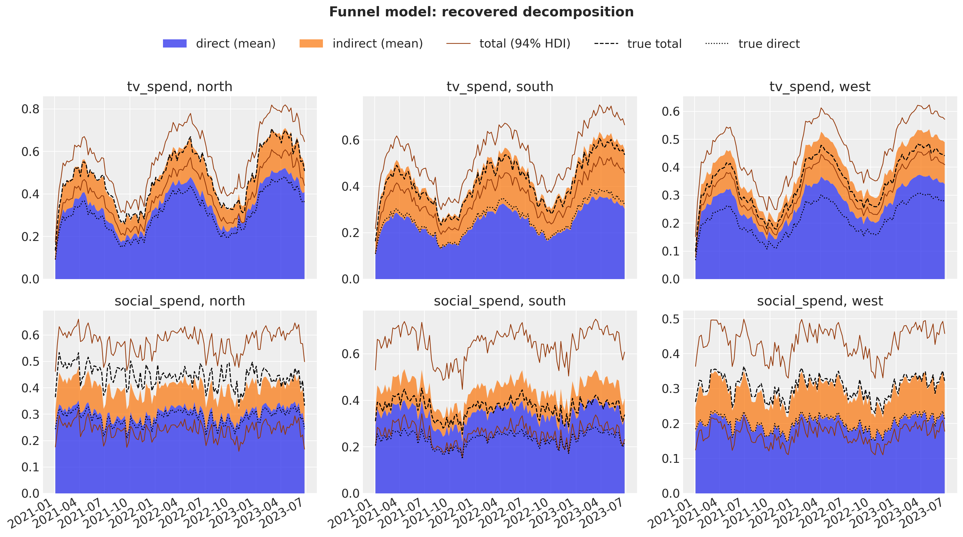
The stack edge is a posterior mean, while the two thin lines bracket a 94% HDI of the same total. They are different summaries of one quantity, so the edge need not sit midway between them. The point of the figure is the split: how much of each channel’s contribution travels directly versus through lower-funnel spend, against the two black reference lines.
Head-to-head: the bias from ignoring the funnel#
Important
Where this lands. Every mediator-blind model pays for the funnel it cannot see, and the bill differs by channel. Naive B (mediator omitted) overstates TV through the shared growth trend. Naive B++ (trend as control) repairs TV and misallocates onto social instead. Naive A (mediator as channel) is not so much wrong as answering the direct-effect question, so it is scored against both benchmarks below.
Finally we compare the six models on the quantity a budget decision actually turns on: the total contribution of each upper-funnel channel. For the naive models the channel contribution is already the counterfactual versus zero spend. For the funnel model we use direct plus the counterfactual indirect effect.
The rows are grouped by estimand, following the d-separation analysis. The models above the separator answer (or claim to answer) the total-effect question. Naive A (mediator as channel) sits below it with the funnel model’s direct path, because the direct effect is the question it actually answers. Every bias annotation names its benchmark.
The figure is a forest plot of means and intervals against the true values, and the ROAS comparison further down wants exactly the same panel, so we write it once:
FOREST_COLORS = ["C2", "C4", "C5", "C6", "C8", "C3", "C0", "C1"]


def forest_panel(ax, rows, reference=None, benchmarks=None, annotate=True):
    """Draw one mean-and-HDI interval per row, with optional reference lines.

    ``rows`` maps a label to a posterior ``DataArray``. ``reference`` maps a
    benchmark name to ``(value, style)`` and is drawn as a full-height vertical
    line. ``benchmarks`` maps a row label to the benchmark its bias annotation is
    measured against (default: the first ``reference`` entry); the annotation
    names its benchmark so the same figure can mix estimands without ambiguity.
    """
    labels = list(rows)
    benchmarks = benchmarks or {}
    for i, label in enumerate(labels):
        draws = rows[label]
        lo, hi = hdi_bounds(draws)
        mean = float(draws.mean())
        color = FOREST_COLORS[i % len(FOREST_COLORS)]
        ax.plot([float(lo), float(hi)], [i, i], color=color, lw=3.5, alpha=0.65)
        ax.plot([mean], [i], "o", color=color, ms=9)
        if annotate and reference:
            key = benchmarks.get(label, next(iter(reference)))
            benchmark = reference[key][0]
            ax.annotate(
                f"{mean / benchmark - 1:+.0%} vs {key}",
                (mean, i),
                textcoords="offset points",
                xytext=(0, -15),
                ha="center",
                va="top",
                fontsize=8,
                bbox={
                    "boxstyle": "round,pad=0.15",
                    "fc": "white",
                    "ec": "none",
                    "alpha": 0.75,
                },
            )
    for name, (value, style) in (reference or {}).items():
        ax.axvline(value, label=f"true {name}", **style)
    ax.set_yticks(range(len(labels)))
    ax.set_yticklabels(labels)
    ax.set_ylim(-0.7, len(labels) - 0.3)
    ax.invert_yaxis()


TRUE_STYLE = {
    "total": {"color": "black", "linestyle": "--", "linewidth": 2},
    "direct": {"color": "gray", "linestyle": ":", "linewidth": 2},
}
def total_contribution(model: MMM, channel: str) -> xr.DataArray:
    """Mean-over-time total contribution of ``channel`` for a naive model."""
    return (
        model.idata.posterior["channel_contribution_original_scale"]
        .sel(channel=channel)
        .mean(dim="date")
    )


estimates = {
    "Naive B (mediator omitted)": lambda ch: total_contribution(naive_b, ch),
    "Naive B+ (demand as control)": lambda ch: total_contribution(naive_bplus, ch),
    "Naive B++ (trend as control)": lambda ch: total_contribution(naive_bpp, ch),
    "Naive C (indicator as channel)": lambda ch: total_contribution(naive_c, ch),
    "Funnel (total)": lambda ch: total_post.sel(channel=ch).mean(dim="date"),
    "Naive A (mediator as channel)": lambda ch: total_contribution(naive_a, ch),
    "Funnel (direct only)": lambda ch: direct_post.sel(channel=ch).mean(dim="date"),
}
CONTRIBUTION_BENCHMARKS = {
    "Naive A (mediator as channel)": "direct",
    "Funnel (direct only)": "direct",
}

truth_mean = data["total_true"].mean("date")
direct_truth_mean = data["direct_true"].mean("date")
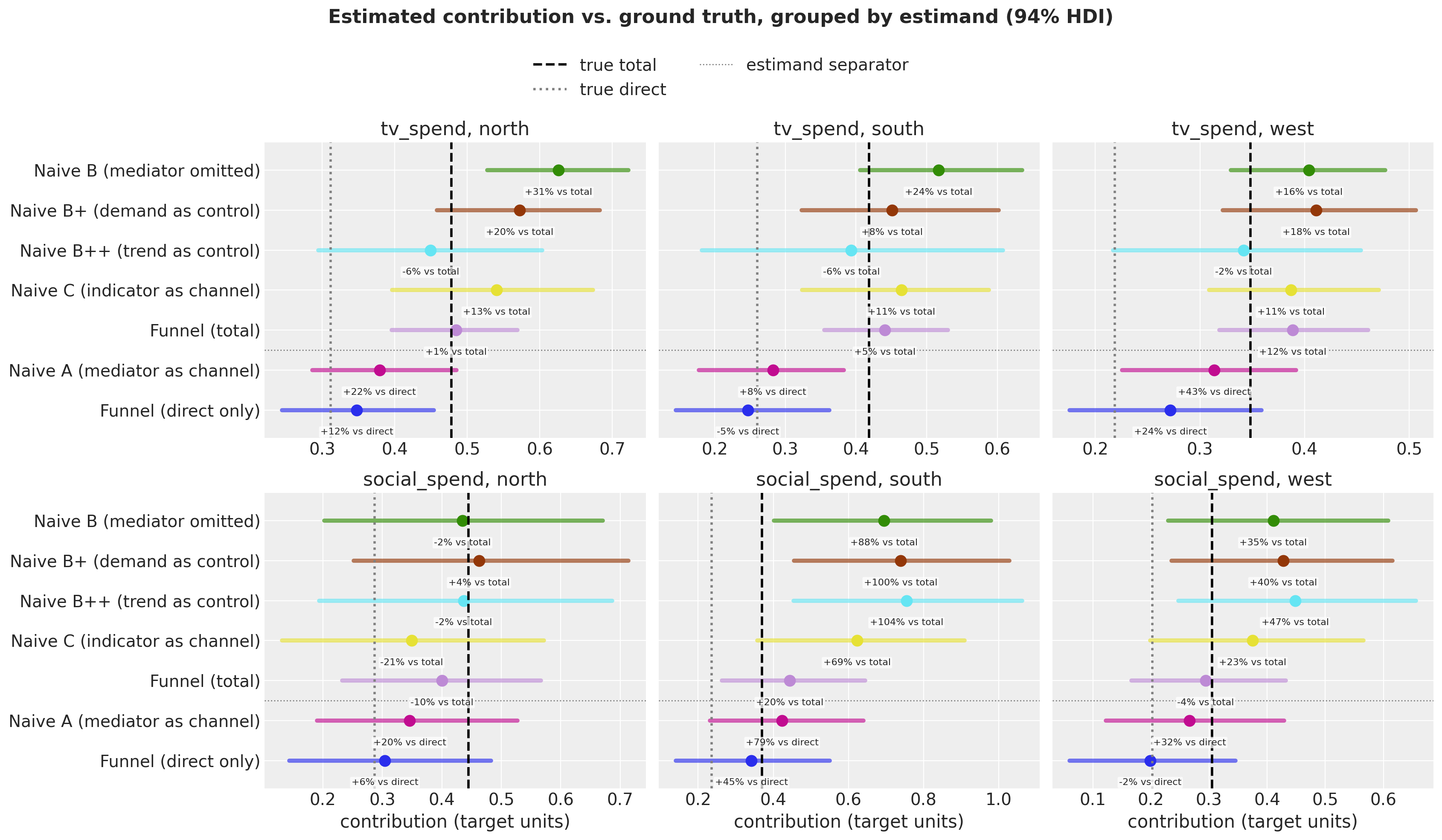
Each verdict from the d-separation table now has an empirical face, and the two channels put two different failure mechanisms on display.
Naive B (mediator omitted) overstates TV, and the trend is why. TV is the channel whose residual correlation with category demand survived the seasonal projection at +0.63 to +0.67. It comes out overstated in every geo (+16.0% to +30.8%). This is textbook confounding: trending category demand, routed through the mediator into the target, credited to the one regressor that also trends.
Both candidate fixes do repair TV, and the graph’s ranking of them is inverted. Naive B++ (trend as control) conditions on the trend itself, exactly where the graph put one of the two forks. Its TV estimates land within a few points of the truth, just past it on the other side (-6.0% to -1.9%). Naive B+ (demand as control) conditions downstream on the category index: the specification the graph nominated, because it blocks the noise fork too. It recovers only part of the same correction (TV at +7.9% to +19.7%, and in west it nudges TV slightly further out rather than back).
So the adjustment set with the weaker formal credential does the better empirical job here. Its linear control competes with the flexible response curves for the same variance. As the arithmetic below shows, a trend the curves cannot mimic is won more decisively than a category index they can. Graph validity ranks specifications only up to functional form; it never promised more.
Social is the twist. Naive B wildly overstates it in two geos (+88.1% in south, +34.5% in west) against a near-exact -2.2% in north, and both fixes make it worse on average (mean |error| 41.6% to 48.1% and 51.0%). Social’s backdoor is graphically open, exactly like TV’s: \(t \to U_2\) is in the graph, and the symmetry check above says the verdicts are identical with social as the treatment. But it is numerically immaterial. Its residual correlation with demand was at noise level (\(|r| \le 0.12\)) before any fix was applied.
That is a statement about the two observable strands, and worth keeping separate from the third. On this draw the drivers’ shared noise is essentially a social-side phenomenon: pooled -0.126 on social against +0.007 on TV, and north social, at -0.180, is the biggest entry in that table. “On this draw” is doing real work in that sentence. The claims around it are design properties, but which channel the unobservable strand lands harder on is exactly the kind of number the floor discussion said a redraw reshuffles, sign included. It cannot be what inflates social, because the sign is wrong: a negative confounding correlation does not manufacture a positive bias. But here the strand no regressor spans is, on this channel, the larger one.
So social’s overstatement is not confounding in any quantitative sense. It is the omitted mediated path. The demand pool that upper-funnel spend fills is missing from every naive model, so its contribution has to land somewhere, and it lands disproportionately on social. Why it prefers social is a claim about where the likelihood puts the mass, so we price it in target units below rather than leave it as an assertion. No adjustment set can address the misallocation: no backdoor an adjustment set could reach is material here, and the one it cannot reach points the other way. What is left is the model family, which simply cannot represent one shared saturating pool as a sum of per-channel curves. D-separation speaks about which variables you need, never about how they must enter. And, being binary, it cannot tell you that one open backdoor is worth 0.65 and the other 0.1.
So the graph’s guess from the correlation table was half right. The bias the graph could see and the measurement said was material (TV’s open backdoor) did land on TV, and adjustment removed it. The larger bias landed on the channel whose backdoor was numerically empty, and adjustment could not touch it.
Naive C sits between Naive A and Naive B, and inherits from both. Branded search is a near-perfect proxy for latent demand. Conditioning on it blocks the mediated path the way Naive A does, but only partially, while leaving TV’s backdoor as wide open as Naive B does. The two pull opposite ways. On TV they settle into a near-uniform +11.0% to +13.0%, averaging almost exactly half of B’s +23.5%: the partial block gives back about half of B’s inflation and no more. That column is the tidy part. Social is where the leftover lands, and it swings from -21.4% in north through +22.9% in west to +68.6% in south, changing sign on the way. A model whose error is a constant on one channel and a sign-changing spread on the other is arguably more dangerous than one that is wrong the same way everywhere. The tidy column invites exactly the correction factor the other column would defeat.
Naive A, read against its own estimand, is a different model. Against the total effect it understates TV badly: the blocked indirect path. Against the true direct effect (the dotted line, its annotation benchmark below the separator) it covers five of six cells, though with a mean error near 34%. It is a rough direct-effect estimator, not a clean one. The d-separation analysis said as much, since it conditions on the noisy observation \(M\) rather than the structural \(M^{*}\). The lesson is not “Naive A is broken” but “Naive A answers a question nobody asked it, and answers it only approximately”.
A third thing sits in the picture: the direct-versus-mediated trade-off the recovery table found in the funnel model’s own posterior. It is not a separable contributor, as the absolute-bias section below shows, but it has a structural half and a draw half. The structural half was named when that table was read. Both paths originate at the same upper-funnel spend, so how the response splits between them is only weakly identified, and that weak identification leaves room for a sizeable per-cell residual on any draw. Which cells it lands on, and how hard, is the draw’s half. It is not a specification failure, and no conditioning choice removes it; the funnel model has the right structure and still carries it.
Whether the naive models carry the same trade-off is a separate question, and the honest answer is that nothing here settles it. The absolute-bias section below reaches for the one ruler that could place a single model’s carryover on a direct-to-mediated ladder. It finds the ladder narrower than the interval it would have to be read against, so neither a subtraction nor a floor is licensed. That is why the section keeps the funnel model’s residual only as a reference point for what a right-structure model still carries.
None of these biases is a uniform shift you could correct with a fudge factor. The two mechanisms respond to different remedies: one to a control column, the other only to modelling the funnel. We quantify all of it below, where a single number per model replaces eyeballing these intervals.
The claim that Naive B+’s control wins only part of the shared trend variance deserves its arithmetic:
What should these coefficients be? In the true DGP a sustained +1 in category demand raises latent demand by \(\gamma_g\), hence \(M^{*}\) by \(\gamma_g\): the geometric adstock is normalized, so a sustained shift passes through with total weight one. The target then rises by \(\gamma_g\) times the slope of the true conversion curve at its operating point. LogisticSaturation is \(\beta \tanh(\lambda x / 2)\), so that slope is \(\beta\,(\lambda/2)/\cosh^{2}(\lambda x / 2)\), averaged pointwise over the adstocked \(M^{*}\) series.
Naive B++’s control is the calendar trend itself, so its anchor runs one step further back. A sustained +1 in \(t\) raises the category index by its trend loading times the softplus derivative, times the Jacobian of the index’s rescaling. It then reaches the target through the identical demand \(\to M^{*} \to\) conversion chain, under the same mean-of-slope convention, so the two anchors are comparable.
Note
Two caveats on the anchors. The normalized adstock passes a sustained shift through with total weight one only from week l_max on; the zero-padded start passes slightly less, worth under half a percent here. And averaging the pointwise slope gives the mean of the slope, not the slope at the mean (no Jensen gap). But it is still not the regression’s own estimand, which weights the slope by where the variance sits: same order of magnitude, not the identical number.
adstock_weights = np.power(true["adstock_lf_alpha"][None, :], np.arange(l_max)[:, None])
adstock_weights /= adstock_weights.sum(axis=0)
mstar = data["lf_spend_true"].transpose("date", "geo").to_numpy()
adstocked_mstar = np.stack(
    [
        np.convolve(mstar[:, g], adstock_weights[:, g])[: len(mstar)]
        for g in range(len(geos))
    ],
    axis=1,
)
lam_lf = float(true["sat_lf_lam"])
pointwise_slope = (
    true["sat_lf_beta"] * (lam_lf / 2) / np.cosh(lam_lf * adstocked_mstar / 2) ** 2
)
conversion_slope = pointwise_slope.mean(axis=0)

# The softplus derivative is recovered as 1 - exp(-softplus_output), on the
# index with the geo rescaling undone, the same division the noise cell
# applies before inverting.
softplus_out = x_data[..., 2] / geo_size[None, :]
softplus_slope = (1.0 - np.exp(-softplus_out)).mean(axis=0) * (
    geo_size / x_data[..., 2].max()
)
implied_slopes = {
    "Naive B+": true["funnel_gamma"] * conversion_slope,
    "Naive B++": true["funnel_gamma"]
    * trend[drivers.index("category_demand")]
    * softplus_slope
    * conversion_slope,
}
control_of = {
    "Naive B+": (naive_bplus, "category_demand"),
    "Naive B++": (naive_bpp, "t"),
}
# The default control prior is Normal(0, 2) on the *scaled* target, so its sd in
# the original units the implied slope lives in is 2 * target_scale.
control_blocks = {}
for control_label, (control_model, control_name) in control_of.items():
    control_scale = control_model.idata.constant_data["target_scale"]
    gamma_scaled = (
        control_model.idata.posterior["gamma_control"].sel(control=control_name)
        * control_scale
    )
    post_mean = gamma_scaled.mean(dim=["chain", "draw"]).to_series()
    post_sd = gamma_scaled.std(dim=["chain", "draw"]).to_series()
    implied = pd.Series(implied_slopes[control_label], index=pd.Index(geos, name="geo"))
    prior_sd = (2.0 * control_scale).to_series()
    control_blocks[control_label] = pd.DataFrame(
        {
            "posterior mean (target scale)": post_mean,
            "implied true slope": implied,
            "posterior sd (target scale)": post_sd,
            "sd from implied": (post_mean - implied).abs() / post_sd,
            "sd from zero": post_mean.abs() / post_sd,
            "prior sd (target scale)": prior_sd,
            "prior sd / implied": prior_sd / implied,
        }
    )
summary = pd.concat(control_blocks, names=["model"])
summary.style.format(
    {col: "{:.3f}" for col in summary.columns} | {"prior sd / implied": "{:.0f}x"}
)
| posterior mean (target scale) | implied true slope | posterior sd (target scale) | sd from implied | sd from zero | prior sd (target scale) | prior sd / implied | ||
|---|---|---|---|---|---|---|---|---|
| model | geo | |||||||
| Naive B+ | north | 0.137 | 0.118 | 0.059 | 0.320 | 2.326 | 4.367 | 37x |
| south | 0.205 | 0.119 | 0.087 | 0.994 | 2.362 | 3.530 | 30x | |
| west | 0.026 | 0.098 | 0.108 | 0.662 | 0.243 | 2.561 | 26x | |
| Naive B++ | north | 0.146 | 0.031 | 0.038 | 3.024 | 3.850 | 4.367 | 139x |
| south | 0.094 | 0.022 | 0.039 | 1.844 | 2.408 | 3.530 | 161x | |
| west | 0.058 | 0.012 | 0.026 | 1.753 | 2.210 | 2.561 | 216x |
The arithmetic explains why Naive B+ recovers only part of TV’s correction. The correct linear effect of a unit of category demand on the target is small, about a tenth of a unit (the implied-slope column), because a unit of demand converts through the saturating lower-funnel curve. The posterior means scatter around that implied slope rather than tracking it: above it in north and south, well below it in west, though each lands within about one posterior sd of the anchor. The sd-from-zero column is the honest one. Two of the three cells sit more than two posterior sds from zero, so the control is doing measurable work there. west’s sits a quarter of an sd away, which is a control the data cannot tell apart from an omitted column. At this sample size the diagnostic cannot distinguish a control doing its full job from one doing half of it, or, in west, from one doing nothing.
(This is also why we do not read the posterior-to-prior shrinkage as strength here the way we did for \(\lambda\). The default \(\mathrm{Normal}(0, 2)\) control prior lives on the scaled target, so the comparison has to be made in one currency. In original units its sd is \(2 \cdot \texttt{target\_scale}\), tens of times wider than the implied slope in Naive B+’s rows of the last column above. A posterior that has shrunk to a few percent of that is still wide relative to the number it is trying to measure.)
Naive B++’s rows tell the complementary story, and they are why the inversion has a mechanism rather than a moral. Its implied slope is smaller still, because its anchor chains through the category index’s trend loading, the softplus derivative, and the rescaling. Yet its posterior means sit far above that anchor in all three geos: 0.146, 0.094 and 0.058 against 0.031, 0.022 and 0.012, four to five times the demand-path prediction, with posterior sds between about two thirds and a quarter of Naive B+’s. A linear column in \(t\) wins the trend strand outright, more than the demand-path anchor alone predicts, consistent with it also absorbing trend co-movement the response curves cannot bend to mimic. The category index, competing with those same curves for shared variance, recovers only part of its own slope. That is the asymmetry the adjustment section promised as arithmetic.
The fit resolves what the coefficient alone cannot. The control and the flexible TV response curve compete for the same trend variance, and the posterior splits it between them. In north and south, B+’s TV estimates land part of the way from Naive B’s toward Naive B++’s (+30.8% to +19.7% to -6.0%, and +23.7% to +7.9% to -6.0%). In west, where the control’s coefficient sits a quarter of a posterior sd from zero, B+ barely moves at all, and what movement there is goes the wrong way (+16.0% to +18.0%): the same story told in a single cell. The trend control in B++ wins the same contest more decisively, because a curve has to bend to mimic a trend while \(t\) enters linearly. That is why the cheaper, only-conditionally-valid fix closes TV’s gap more fully than the one the graph nominated. Both observations say the same thing. A formally valid control can be estimated about right and still be under-deployed, because validity says nothing about how strongly the likelihood will lean on a linear term when nonlinear alternatives can partially mimic it. What neither control touches, as the tables below quantify, is the social side. There the backdoor was open on the graph but empty in the measurement, so there was no material confounding for either of them to remove.
ROAS, nationally and per geo#
Important
Where this lands. The ROAS ordering reproduces the contribution ordering above; what is new here is the denominator. Upper-funnel activity induces lower-funnel spend that someone has to authorise, and only a model that sees the funnel can price it, so Funnel (total) and the induced-spend row answer two different budget questions.
Budget decisions key off return on ad spend, so let us express the same comparison that way. All estimates use the same definition (contribution summed over the observed weeks, divided by spend over those same weeks) so that any difference between them is structural rather than definitional.
One convention needs naming before any number is read. The standard rows below divide by upper-funnel spend alone: they report return per upper-funnel dollar, treating the lower-funnel spend that upper-funnel activity induces as free. That is not an innocent choice here. The coefficient on \(D\) in the \(M^{*}\) equation is exactly one, so every unit of demand a channel creates is a unit of incremental lower-funnel spend someone has to authorise. With roughly a third of each channel’s effect travelling that path, it is not a rounding issue either. The funnel model is the only one that can price that induced spend. So alongside Funnel (total) we also report a row that adds it to the denominator: \(\Delta y \,/\, (\text{channel spend} + \Delta M^{*})\).
One bookkeeping assumption underlies that row: all spend series are denominated in the same currency, so upper-funnel dollars and induced lower-funnel dollars can be added in one denominator. On real data that is automatic. In this synthetic DGP the “exchange rate” between a TV unit and a lower-funnel unit is set by each series’ max-normalization, exactly as arbitrary as it sounds. So read the induced-spend row as a demonstration of the accounting, not of a meaningful price.
spend = data[channels].to_array("channel").sum("date")


def incrementality_roas(model: MMM) -> xr.DataArray:
    """All-time ROAS via the incrementality module's spend counterfactual.

    For a model whose effects opted in, this is the total effect.
    """
    return model.incrementality.contribution_over_spend(frequency="all_time").sel(
        channel=channels
    )


def roas_from(contribution: xr.DataArray) -> xr.DataArray:
    """All-time ROAS: summed contribution over summed spend, per channel and geo."""
    return contribution.sel(channel=channels).sum(dim="date") / spend


# Denominator including each channel's induced lower-funnel spend. The denominator
# is itself a posterior quantity: the model estimates how much M* the channel moved.
denom_incl = spend + induced_spend_post.sum(dim="date")

# `FunnelEffect` opted in through `incrementality_spec`, so for the funnel model
# the built-in follows the spend counterfactual down both paths and returns the
# total (direct + mediated). The direct-only row is assembled from the posterior
# channel contributions instead, and only the induced-spend denominator still
# needs the manual counterfactual: the module's increment is in target units,
# while the induced spend is a spend series it does not report.
roas = {
    "Naive B (mediator omitted)": incrementality_roas(naive_b),
    "Naive B+ (demand as control)": incrementality_roas(naive_bplus),
    "Naive B++ (trend as control)": incrementality_roas(naive_bpp),
    "Naive C (indicator as channel)": incrementality_roas(naive_c),
    "Funnel (total)": incrementality_roas(funnel),
    "Funnel (total / all incremental spend)": (
        total_post.sel(channel=channels).sum(dim="date") / denom_incl
    ),
    "Naive A (mediator as channel)": incrementality_roas(naive_a),
    "Funnel (direct only)": roas_from(
        funnel.idata.posterior["channel_contribution_original_scale"]
    ),
}
ROAS_BENCHMARKS = {
    "Funnel (total / all incremental spend)": "total incl. LF",
    "Naive A (mediator as channel)": "direct",
    "Funnel (direct only)": "direct",
}

true_total_roas = data["total_true"].sum("date") / spend
true_direct_roas = data["direct_true"].sum("date") / spend
true_denom_incl = spend + data["induced_spend_true"].sum("date")
true_incl_roas = data["total_true"].sum("date") / true_denom_incl
Note
Every row above comes from the same built-in call, mmm.incrementality.contribution_over_spend(frequency="all_time"), which runs a per-channel on/off spend counterfactual. For the naive models that is simply their channel ROAS. For the funnel model, FunnelEffect opted in through incrementality_spec, so the counterfactual is followed down both paths, and Funnel (total) is the module’s own number rather than a hand-assembled one. Had the effect not opted in, the call would raise instead of quietly reporting the direct path as if it were the whole thing. The Funnel (direct only) row is therefore the one assembled by hand now, and only the induced-spend denominator still needs the posterior counterfactual from the previous section.
The check below compares the module’s total against the direct-plus-indirect ROAS assembled by hand there. The agreement to printed precision is necessary, not lucky. With frequency="all_time" the evaluation window is the whole series, so there is nothing for the built-in’s carry-over extension to extend into: the windowed attribution and the whole-series zeroing compute the same difference, draw by draw, up to float roundoff. The carry-over extension only bites when a window boundary falls inside the data, as the yearly breakdown below shows.
manual_total = roas_from(total_post)

pd.DataFrame(
    {
        "incrementality, all_time (direct + mediated)": roas["Funnel (total)"]
        .mean(dim=["chain", "draw"])
        .transpose("channel", "geo")
        .to_series(),
        "manual counterfactual (direct + indirect)": manual_total.mean(
            dim=["chain", "draw"]
        )
        .transpose("channel", "geo")
        .to_series(),
    }
).style.format("{:.4f}")
| incrementality, all_time (direct + mediated) | manual counterfactual (direct + indirect) | ||
|---|---|---|---|
| channel | geo | ||
| tv_spend | north | 0.4021 | 0.4021 |
| south | 0.5225 | 0.5225 | |
| west | 0.7000 | 0.7000 | |
| social_spend | north | 0.5089 | 0.5089 |
| south | 0.7907 | 0.7907 | |
| west | 0.8065 | 0.8065 |
To see include_carryover actually doing something, ask for yearly windows. Now 2021 and 2022 end mid-data, and the carryover option credits each year with the response its spend leaves in flight afterwards. That reach is l_max weeks of direct adstock plus the further weeks the mediator’s second adstock adds: exactly the window the declared additional_carryover_lags sized. Since the effect opted in, these yearly figures are totals (direct + mediated), like the all-time rows above:
# The same integer seed for both calls, so they subsample the same posterior
# draws and the difference column is not polluted by Monte Carlo noise. A shared
# `rng` would not do here: the subsampling helper consumes the generator it is
# handed, so the second call would land on different draws.
yearly_with = funnel.incrementality.contribution_over_spend(
    frequency="yearly",
    num_samples=500,
    random_state=seed,
)
yearly_without = funnel.incrementality.contribution_over_spend(
    frequency="yearly",
    include_carryover=False,
    num_samples=500,
    random_state=seed,
)

yearly = pd.DataFrame(
    {
        "with carryover": yearly_with.mean(dim=["chain", "draw"])
        .sel(channel=channels)
        .to_series(),
        "without": yearly_without.mean(dim=["chain", "draw"])
        .sel(channel=channels)
        .to_series(),
    }
)
yearly["difference"] = yearly["with carryover"] - yearly["without"]
yearly.style.format("{:.4f}")
| with carryover | without | difference | |||
|---|---|---|---|---|---|
| date | channel | geo | |||
| 2021-12-31 00:00:00 | tv_spend | north | 0.4611 | 0.4491 | 0.0120 |
| south | 0.5868 | 0.5717 | 0.0151 | ||
| west | 0.7829 | 0.7643 | 0.0186 | ||
| social_spend | north | 0.5272 | 0.5228 | 0.0044 | |
| south | 0.8189 | 0.8118 | 0.0070 | ||
| west | 0.8215 | 0.8162 | 0.0054 | ||
| 2022-12-31 00:00:00 | tv_spend | north | 0.4113 | 0.4031 | 0.0082 |
| south | 0.5393 | 0.5275 | 0.0118 | ||
| west | 0.7107 | 0.6981 | 0.0125 | ||
| social_spend | north | 0.4971 | 0.4929 | 0.0042 | |
| south | 0.7886 | 0.7810 | 0.0076 | ||
| west | 0.8049 | 0.7969 | 0.0080 | ||
| 2023-12-31 00:00:00 | tv_spend | north | 0.3282 | 0.3282 | 0.0000 |
| south | 0.4251 | 0.4251 | 0.0000 | ||
| west | 0.5756 | 0.5756 | 0.0000 | ||
| social_spend | north | 0.4377 | 0.4377 | 0.0000 | |
| south | 0.6832 | 0.6832 | 0.0000 | ||
| west | 0.6977 | 0.6977 | 0.0000 |
The interior years differ, as they should. Two footnotes stop this table from being misread. The final, partial year’s window ends at the calendar boundary, past the last observation. Its two columns are therefore identical for exactly the reason the all_time columns were: beyond the data there is nothing to extend into. And with carryover on, the yearly windows overlap: each year’s carryout weeks lie inside the next year’s window, so the yearly figures deliberately do not aggregate back to the all-time number.
Nationally#
# National = total contribution over total spend; each row keeps its own
# denominator, so the induced-spend row is weighted by spend *plus* induced spend.
national = {
    label: (da * spend).sum("channel").sum("geo") / spend.sum()
    for label, da in roas.items()
    if label != "Funnel (total / all incremental spend)"
}
national["Funnel (total / all incremental spend)"] = (
    roas["Funnel (total / all incremental spend)"] * denom_incl
).sum(["channel", "geo"]) / denom_incl.sum(["channel", "geo"])
national = {label: national[label] for label in roas}  # restore row order

national_true_total = float((true_total_roas * spend).sum() / spend.sum())
national_true_direct = float((true_direct_roas * spend).sum() / spend.sum())
national_true_incl = float(
    (true_incl_roas * true_denom_incl).sum() / true_denom_incl.sum()
)

fig, ax = plt.subplots(figsize=(11, 6.5))
forest_panel(
    ax,
    national,
    reference={
        "total": (national_true_total, TRUE_STYLE["total"]),
        "direct": (national_true_direct, TRUE_STYLE["direct"]),
        "total incl. LF": (
            national_true_incl,
            {"color": "black", "linestyle": "-.", "linewidth": 1.5, "alpha": 0.6},
        ),
    },
    benchmarks=ROAS_BENCHMARKS,
)
# Estimand separator: total-effect rows above, direct-effect rows below.
ax.axhline(len(national) - 2.5, color="gray", linestyle=":", lw=1)
ax.set_xlabel("ROAS")
ax.legend(loc="lower right")
ax.set_title(
    "Spend-weighted national ROAS by model (94% HDI)",
    fontsize=15,
    fontweight="bold",
)
fig.set_layout_engine("tight")
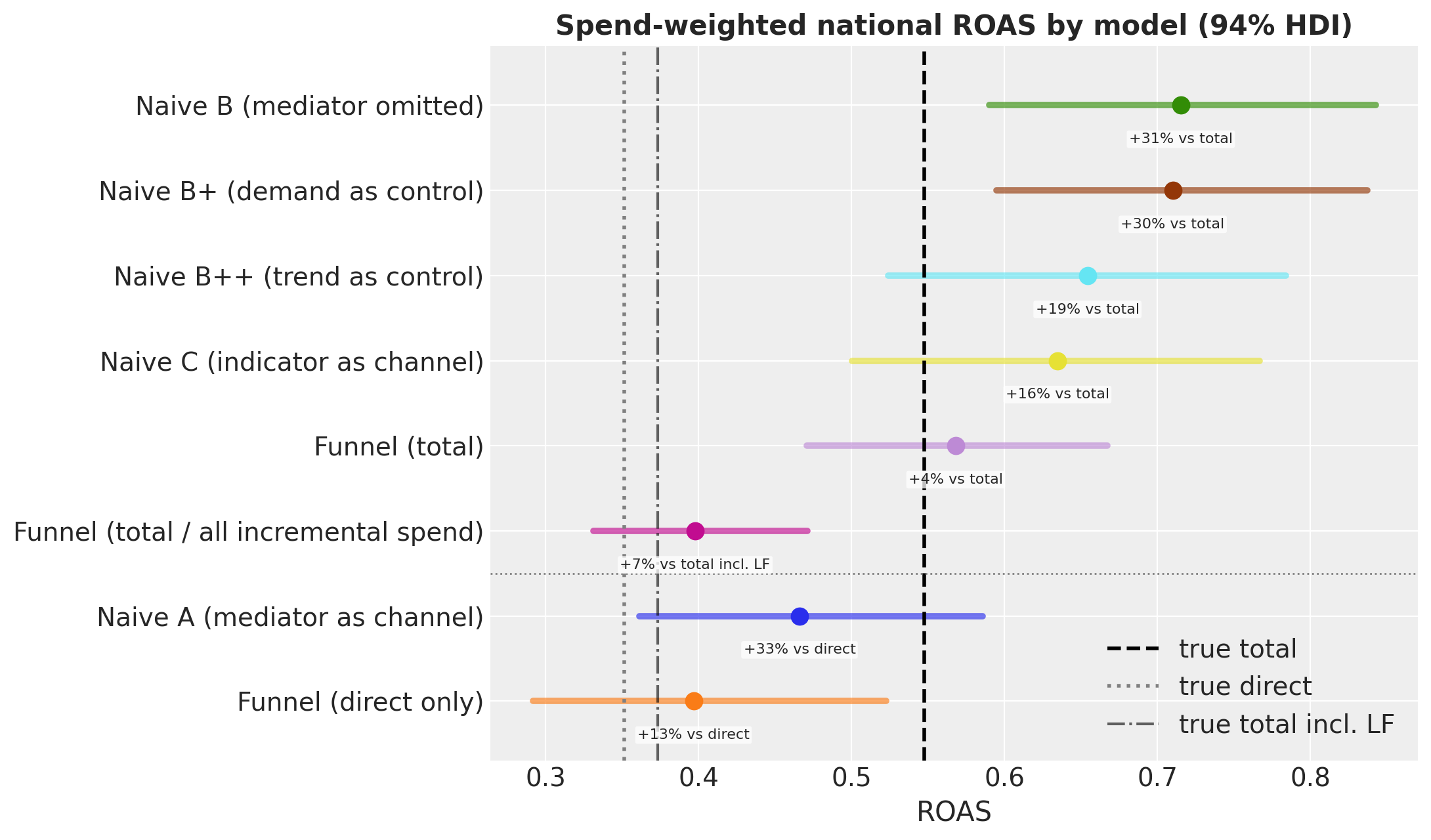
The rows above the separator estimate a total effect. The first five are annotated against the true total (dashed black). The sixth divides the same total contribution by all the incremental money it took, channel spend plus the induced lower-funnel spend, and is annotated against its own benchmark (dash-dotted). The gap between the two funnel rows is the price of the induced spend. The return per upper-funnel dollar and the return per incremental dollar are different questions, and only a model that sees the funnel can answer the second one at all.
Below the separator sit the two direct-effect rows, annotated against the true direct ROAS (dotted grey), including Naive A, per the d-separation analysis: this is the question it actually answers. Neither direct row sits cleanly on the dotted line, and per cell their errors partly offset in the national average. The direct path inherits the same amplitude trade-off the recovery table found, and social in south, the widest seesaw cell there, is also the direct rows’ largest single miss. A correct decomposition is not a magic wand against one dataset’s noise; what it buys is the right estimand and honest uncertainty around it.
Read as a budget input: the naive models disagree with the truth in different directions, and nothing in the models themselves tells you which one you are looking at.
Per geo and channel#
The national number averages over exactly the heterogeneity a geo panel exists to expose, so it is worth breaking out. contribution_over_spend returns (chain, draw, channel, geo) (as does the manual counterfactual feeding the induced-spend row), so no extra computation is needed: only a different view of it.
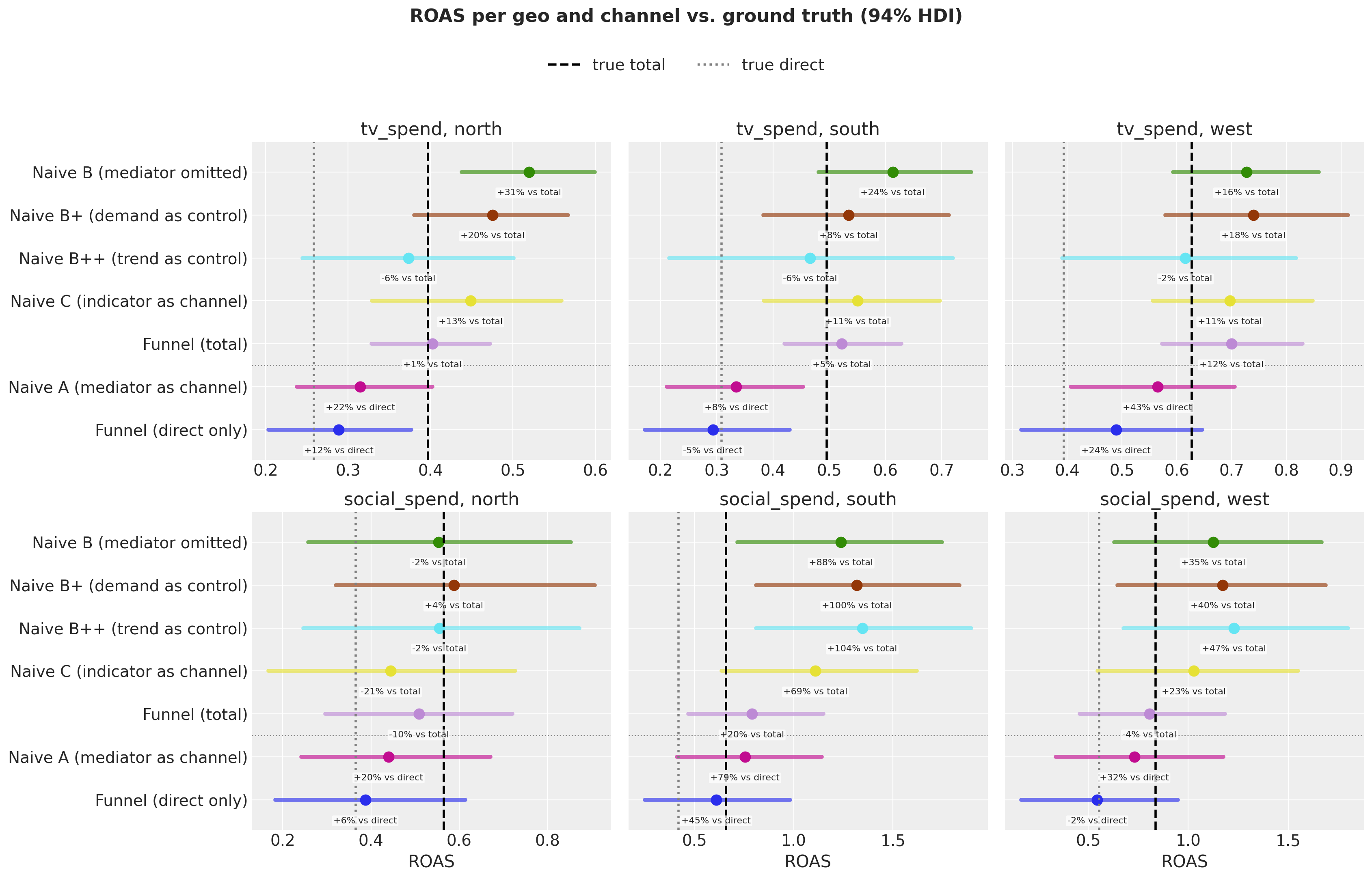
The same comparison as a table of levels, then as bias against the true total:
roas_summary = pd.DataFrame(
    {
        label: da.mean(dim=["chain", "draw"]).transpose("channel", "geo").to_series()
        for label, da in roas.items()
    }
)
roas_summary["true direct"] = true_direct_roas.transpose("channel", "geo").to_series()
roas_summary["true total"] = true_total_roas.transpose("channel", "geo").to_series()
roas_summary["true total incl. LF"] = true_incl_roas.transpose(
    "channel", "geo"
).to_series()
roas_summary.style.format("{:.3f}")
| Naive B (mediator omitted) | Naive B+ (demand as control) | Naive B++ (trend as control) | Naive C (indicator as channel) | Funnel (total) | Funnel (total / all incremental spend) | Naive A (mediator as channel) | Funnel (direct only) | true direct | true total | true total incl. LF | ||
|---|---|---|---|---|---|---|---|---|---|---|---|---|
| channel | geo | |||||||||||
| tv_spend | north | 0.519 | 0.475 | 0.373 | 0.449 | 0.402 | 0.304 | 0.315 | 0.289 | 0.259 | 0.397 | 0.294 |
| south | 0.613 | 0.535 | 0.466 | 0.550 | 0.523 | 0.352 | 0.335 | 0.293 | 0.309 | 0.496 | 0.349 | |
| west | 0.728 | 0.740 | 0.615 | 0.697 | 0.700 | 0.454 | 0.565 | 0.489 | 0.394 | 0.627 | 0.406 | |
| social_spend | north | 0.553 | 0.588 | 0.555 | 0.444 | 0.509 | 0.377 | 0.440 | 0.387 | 0.365 | 0.565 | 0.378 |
| south | 1.239 | 1.318 | 1.345 | 1.110 | 0.791 | 0.568 | 0.755 | 0.610 | 0.421 | 0.659 | 0.428 | |
| west | 1.125 | 1.172 | 1.228 | 1.028 | 0.806 | 0.482 | 0.730 | 0.545 | 0.555 | 0.836 | 0.501 |
The bias table judges every column against the true total. For five of the six that is their own estimand. Naive A (mediator as channel) is included on the same yardstick deliberately, because “mediator as a channel” is how it gets used in practice. Its column shows the cost of misreading it as a total-effect estimate, and its own estimand is scored separately below.
Read Naive A’s summary row with one caution, though. A percentage bias divides by the estimand it is scored against, and the true direct effect is about two thirds of the true total (the indirect shares above run 33.7% to 37.7%). The same absolute error therefore prints smaller against the total than against the direct effect. That accounts for most of the distance between A’s mean |error| in this table and the roughly 34% it scores against its own estimand.
The absolute table below prices these errors without a denominator, and its uncancelled row reproduces this table’s ordering exactly, so A’s flattering rank is no denominator artifact. (On this draw the signed row happens to give that same order; what it distorts is the magnitudes, which is priced where that table is read.) The flattery lives entirely in which estimand the percentage is scored against.
total_estimates = [
    "Naive A (mediator as channel)",
    "Naive B (mediator omitted)",
    "Naive B+ (demand as control)",
    "Naive B++ (trend as control)",
    "Naive C (indicator as channel)",
    "Funnel (total)",
]
bias = roas_summary[total_estimates].div(roas_summary["true total"], axis=0) - 1
bias.loc[("mean |error|", ""), :] = bias.abs().mean()

# The summary row averages across both channels, while the comparison this
# notebook is organised around is per channel: one failure mechanism each.
by_channel_error = bias.loc[channels].abs().groupby(level="channel", sort=False).mean()
by_channel_error.T.style.format("{:.1%}").set_caption("Mean |error| by channel")
| channel | tv_spend | social_spend |
|---|---|---|
| Naive A (mediator as channel) | 21.1% | 16.5% |
| Naive B (mediator omitted) | 23.5% | 41.6% |
| Naive B+ (demand as control) | 15.2% | 48.1% |
| Naive B++ (trend as control) | 4.6% | 51.0% |
| Naive C (indicator as channel) | 11.7% | 37.6% |
| Funnel (total) | 6.1% | 11.2% |
bias.style.background_gradient(
    cmap="RdBu_r", vmin=-0.5, vmax=0.5, subset=pd.IndexSlice[channels, :]
).format("{:+.1%}")
| Naive A (mediator as channel) | Naive B (mediator omitted) | Naive B+ (demand as control) | Naive B++ (trend as control) | Naive C (indicator as channel) | Funnel (total) | ||
|---|---|---|---|---|---|---|---|
| channel | geo | ||||||
| tv_spend | north | -20.8% | +30.8% | +19.7% | -6.0% | +13.0% | +1.3% |
| south | -32.5% | +23.7% | +7.9% | -6.0% | +11.0% | +5.4% | |
| west | -9.9% | +16.0% | +18.0% | -1.9% | +11.1% | +11.6% | |
| social_spend | north | -22.2% | -2.2% | +4.1% | -1.8% | -21.4% | -10.0% |
| south | +14.7% | +88.1% | +100.1% | +104.3% | +68.6% | +20.1% | |
| west | -12.7% | +34.5% | +40.2% | +46.8% | +22.9% | -3.6% | |
| mean |error| | +18.8% | +32.5% | +31.7% | +27.8% | +24.7% | +8.7% |
A percentage bias is a ratio, and the two channels do not share a denominator. Before reading anything into the TV/social contrast, price the same errors in target units: estimated minus true contribution, which is what a budget conversation would actually get wrong:
spend_series = spend.transpose("channel", "geo").to_series()
true_contribution = (
    data["total_true"].sum("date").transpose("channel", "geo").to_series()
)

abs_bias = (
    roas_summary[total_estimates]
    .sub(roas_summary["true total"], axis=0)
    .mul(spend_series, axis=0)
)

by_channel = abs_bias.groupby(level="channel", sort=False).sum().loc[channels]
true_by_channel = (
    true_contribution.groupby(level="channel", sort=False).sum().loc[channels]
)

by_channel.T.style.format("{:+.1f}").set_caption(
    "Signed (estimated - true) contribution, summed over geos; true totals: "
    + ", ".join(f"{ch} {true_by_channel[ch]:.1f}" for ch in channels)
)
| channel | tv_spend | social_spend |
|---|---|---|
| Naive A (mediator as channel) | -35.1 | -10.8 |
| Naive B (mediator omitted) | +39.3 | +54.7 |
| Naive B+ (demand as control) | +24.7 | +66.4 |
| Naive B++ (trend as control) | -7.8 | +67.6 |
| Naive C (indicator as channel) | +19.1 | +29.7 |
| Funnel (total) | +9.0 | +2.4 |
Note
Summing signed biases over geos lets a model’s cells cancel: a column that is wrong in both directions nets to something small. The uncancelled sum below (how much contribution is misstated per cell, regardless of direction) cannot be gamed by a lucky sign. In both tables, totals are summed at full precision and then rounded, so a total can differ from the sum of the printed cells by 0.1.
uncancelled = abs_bias.abs().groupby(level="channel", sort=False).sum().loc[channels]
uncancelled_table = uncancelled.T
uncancelled_table["both channels"] = abs_bias[total_estimates].abs().sum()
uncancelled_table.style.format("{:.1f}").set_caption(
    "Misstated contribution, summed as |bias| per cell over geos"
)
| channel | tv_spend | social_spend | both channels |
|---|---|---|---|
| Naive A (mediator as channel) | 35.1 | 24.9 | 60.0 |
| Naive B (mediator omitted) | 39.3 | 57.3 | 96.5 |
| Naive B+ (demand as control) | 24.7 | 66.4 | 91.0 |
| Naive B++ (trend as control) | 7.8 | 69.7 | 77.5 |
| Naive C (indicator as channel) | 19.1 | 54.4 | 73.5 |
| Funnel (total) | 9.0 | 16.8 | 25.8 |
abs_bias.style.background_gradient(cmap="RdBu_r", vmin=-30, vmax=30).format("{:+.1f}")
| Naive A (mediator as channel) | Naive B (mediator omitted) | Naive B+ (demand as control) | Naive B++ (trend as control) | Naive C (indicator as channel) | Funnel (total) | ||
|---|---|---|---|---|---|---|---|
| channel | geo | ||||||
| tv_spend | north | -12.9 | +19.2 | +12.2 | -3.8 | +8.1 | +0.8 |
| south | -17.7 | +12.9 | +4.3 | -3.2 | +6.0 | +2.9 | |
| west | -4.5 | +7.3 | +8.2 | -0.8 | +5.0 | +5.3 | |
| social_spend | north | -12.8 | -1.3 | +2.3 | -1.0 | -12.4 | -5.8 |
| south | +7.0 | +42.3 | +48.1 | +50.1 | +32.9 | +9.6 | |
| west | -5.0 | +13.7 | +15.9 | +18.6 | +9.1 | -1.4 |
The denominators are not the story. In truth the two channels contribute almost the same amount, 162 against 146: social buys less spend but converts it better. A percentage comparison between them was therefore close to fair already, and the absolute table repeats the percentage table’s verdict without the escape hatch. Naive B (mediator omitted) misallocates about half again as much contribution onto social as onto TV (+54.7 against +39.3). Naive B++ (trend as control), the model that fixes TV, misallocates about nine times as much: 69.7 against 7.8 on the uncancelled row. (Here the two readings agree for B++: its three TV cells run -3.8, -3.2 and -0.8, all the same sign, so nothing cancels.) The likelihood really does prefer social; it is not an artifact of dividing by a smaller number.
The cancellation the note above warns about shows up in the by-channel row itself, and the funnel model is the clearest case. Its social column nets to +2.4, close enough to zero to look like a model that gets social nearly right. Its three social cells (-5.8, +9.6 and -1.4) still misstate 16.8 units between them. Naive C’s social column tells the same story more loudly: +29.7 signed against 54.4 uncancelled, because its cells run -12.4, +32.9 and +9.1. Neither reading changes the ranking on this draw, but the signed row understates both models, and by different amounts.
That is the same warning the coverage discussion below gives about C’s flattering mean percentage, printed here in the one table where the cancellation actually happens. Naive B++ is sign-consistent in every cell (TV all negative, social all positive), so its “nine times” above reads the same either way. Naive B has one small opposite-sign cell in social (north, -1.3), which is the whole gap between its +54.7 and its 57.3.
Two things follow that percentages could not show.
A valid adjustment does not only remove bias, it moves some. Going from Naive B to Naive B+, the set the d-separation table scores valid, takes about 15 units of contribution off TV and puts 12 of them back onto social: most of it. Going to Naive B++, the conditionally-valid trend control, takes 47 units off TV (overshooting the truth into a small understatement) and hands 13 to social: about a quarter of what it removed. Either way a large share of what the control takes off the confounded channel reappears on the unconfounded one. With the mediated pool still missing from the model, the contribution it represents has to be attributed somewhere. Closing the backdoor changes where, not whether.
tilt_params = ["adstock_alpha", "saturation_lam"]
social_index = channels.index("social_spend")

tilt_cols = pd.MultiIndex.from_product([tilt_params, ["mean", "sd"]])
tilt_rows = {
    "true": [
        float(true["adstock_alpha"][social_index]),
        np.nan,
        float(true["saturation_lam"][social_index]),
        np.nan,
    ]
}
for label, model in models.items():
    posterior = model.idata.posterior
    row = []
    for param in tilt_params:
        draws = posterior[param].sel(channel="social_spend")
        row += [float(draws.mean()), float(draws.std())]
    tilt_rows[label] = row

pd.DataFrame.from_dict(tilt_rows, orient="index", columns=tilt_cols).style.format(
    "{:.3f}", na_rep=""
).set_caption("Pooled direct-path parameters on social_spend")
| adstock_alpha | saturation_lam | |||
|---|---|---|---|---|
| mean | sd | mean | sd | |
| true | 0.300 | 4.000 | ||
| Naive A | 0.343 | 0.068 | 4.145 | 0.696 |
| Naive B | 0.403 | 0.053 | 4.445 | 0.609 |
| Naive B+ | 0.423 | 0.053 | 4.530 | 0.573 |
| Naive B++ | 0.458 | 0.057 | 4.626 | 0.618 |
| Naive C | 0.384 | 0.061 | 4.310 | 0.659 |
| Funnel | 0.318 | 0.079 | 3.974 | 0.821 |
The mean-lag ruler below is computed from the true kernels rather than asserted. Mean-lag matching asks what single geometric alpha carries the same average delay as two references: the direct path alone, and a curve forced to also absorb the mediated response, whose carryover is the upper-funnel adstock composed with the lower-funnel one.
Note
The ruler is a kernel-shape yardstick: an order-of-size prediction, not a likelihood fit. Only in the funnel model is adstock_alpha purely a direct-path parameter; in a naive model it measures whatever the curve was asked to absorb.
kernel_lags = np.arange(l_max)
alpha_true = float(true["adstock_alpha"][social_index])


def normalized_kernel(alpha):
    weights = alpha**kernel_lags
    return weights / weights.sum()


def kernel_mean_lag(kernel):
    return float((kernel_lags[: len(kernel)] * kernel).sum())


def alpha_with_mean_lag(target_lag):
    low, high = 0.001, 0.999
    for _ in range(60):
        mid = (low + high) / 2
        if kernel_mean_lag(normalized_kernel(mid)) < target_lag:
            low = mid
        else:
            high = mid
    return (low + high) / 2


direct_lag = kernel_mean_lag(normalized_kernel(alpha_true))
indirect_share = (
    (data["indirect_true"].mean("date") / data["total_true"].mean("date"))
    .sel(channel="social_spend")
    .to_numpy()
)
uf_kernel = normalized_kernel(float(true["adstock_uf_alpha"][social_index]))
mediated_lags = []
for lf_alpha in true["adstock_lf_alpha"]:
    mediated_kernel = np.convolve(uf_kernel, normalized_kernel(lf_alpha))[:l_max]
    mediated_lags.append(kernel_mean_lag(mediated_kernel / mediated_kernel.sum()))

blend_lags = [
    (1 - s) * direct_lag + s * m
    for s, m in zip(indirect_share, mediated_lags, strict=True)
]

pd.DataFrame(
    [
        [alpha_true] * len(geos),
        [alpha_with_mean_lag(lag) for lag in blend_lags],
        [alpha_with_mean_lag(lag) for lag in mediated_lags],
    ],
    index=[
        "direct path alone",
        "blend at the true indirect share",
        "mediated path alone",
    ],
    columns=pd.Index(geos, name="geo"),
).style.format("{:.3f}").set_caption(
    "Mean-lag ruler for the carryover column (alpha equivalents; "
    "the direct row is geo-independent)"
)
| geo | north | south | west |
|---|---|---|---|
| direct path alone | 0.300 | 0.300 | 0.300 |
| blend at the true indirect share | 0.397 | 0.384 | 0.367 |
| mediated path alone | 0.527 | 0.498 | 0.470 |
The funnel model’s 16.8 is a reference point: not a floor, and not a share. It is the smallest social error in the comparison on either reading (+2.4 signed, 16.8 uncancelled). The signed figure flatters it for the reason the caution above gives: its three social cells run -5.8, +9.6 and -1.4. Naive A is next at -10.8 signed and 24.9 uncancelled, and it does not get there by being closer to right. A blocks the mediated path outright, so it nets an omitted-pool overshoot against a blocked-path undershoot. What makes 16.8 worth staring at is structure, not rank: it is what the one correctly specified model in the comparison still carries on this draw.
The tempting next step is to subtract it from the naive models’ errors and call the remainder misallocation. The cell above is there to say why that has no license, and the reason is sharper than a caveat. Read the carryover column against the ruler printed under it. The mediated path carries its own, longer carryover: an upper-funnel adstock composed with a lower-funnel one. A single channel curve forced to stand in for both paths should therefore inherit a longer blend. The ruler prices that pull: from 0.300 for the direct path alone, through 0.397/0.384/0.367 for a blend at the true indirect share, to 0.470-0.527 for the mediated path alone. The caveat the cell states still applies: a kernel-shape yardstick, an order of size rather than a fit.
Important
Three ruler rows span about a fifth of an alpha. The recovery table above prints the funnel model’s adstock_alpha[social_spend] with a 94% interval of 0.175 to 0.468: wider than the whole ruler, covering the direct row and the blend row and stopping just short of the mediated one. No single model can be placed on a row of this ruler. There is no “the funnel model sits at the direct row, therefore the excess above it is absorption” reading available, in either direction. The quantity a subtraction would need is the one quantity this notebook cannot measure.
What the ruler can still do is order models, which needs the gaps and not the levels. The order it prints is, end to end, the one the mechanism predicts. The funnel model represents the mediated response explicitly, so its channel curve carries the direct path only, and it is lowest at 0.318. Naive A blocks the mediated path by conditioning on the mediator itself and comes next at 0.343. It sits a little above the funnel model because what it conditions on is the noisy observation \(M\), and because \(M^{*} = D + \lambda B\) drags the budget wedge in with it. Naive C blocks only part of the path through the demand proxy, so it retains some mediated response to absorb and sits above both at 0.384. The three that omit the mediator outright sit above all of them: Naive B at 0.403, Naive B+ at 0.423 and Naive B++ at 0.458.
That ordering is a second readout of the misallocation, in kernel shape rather than in target units. Nothing printed licenses treating the increment above the funnel model as a shared tilt waiting to be netted out, which is all the refusal of the subtraction needs. And one gap in the ordering is not absorption at all. The B-family’s internal 0.403 to 0.423 to 0.458 cannot be, since all three omit the mediator identically. It tracks how much of the trend strand each specification closes, the same variance migration the adjustment section describes, and it runs in the same direction as their 54.7 to 66.4 to 67.6 in target units.
The curvature column sorts the six into exactly the same order (3.974, 4.145 and 4.310 against 4.445, 4.530 and 4.626), which is worth taking as corroboration rather than as a second measurement. Its levels are unplaceable for exactly the reason above. And the B-family is one specification plus a control column, near-forced to cluster, so part of the partition is three models being siblings.
One honesty note carries both columns. The printed sds price each model’s uncertainty about the truth, which is the comparison that defeats placing a model on a row. They do not price the model-to-model differences, which on a single dataset are fixed numbers rather than draws from anyone’s posterior. The ordering claims lean on the second, the refusal to place leans on the first, and neither borrows the other’s ruler.
What survives is a caution about the ceiling rather than a bound above a floor. A model with the right structure still misstates social by 16.8 units here, so Naive B’s 57.3 and Naive B++’s 69.7 must not be read as pure misallocation. But nothing printed licenses splitting either number into a draw part and a specification part. What is printed cuts the other way. The coverage table below has the funnel model covering all three of its social cells, at interval widths 0.425, 0.681 and 0.728, despite errors the bias table above prices at -10.0%, +20.1% and -3.6%. Those 16.8 units are posterior-mean offsets lying entirely inside the model’s own reported intervals, not a residual with a magnitude waiting to be netted out.
A point estimate being off is one thing; being confidently off is worse. The tables below ask, for every geo and channel, whether each model’s 94% HDI actually contains the true total ROAS, and how wide those intervals had to be. One caveat before reading it: these are six correlated cells from a single simulated dataset. Treat the counts as a sanity check, not a calibration study; actual interval calibration needs replicate datasets, which is out of scope for a docs example.
coverage_rows = []
for c in channels:
    for g in geos:
        truth = float(true_total_roas.sel(channel=c, geo=g))
        row = {}
        for label in total_estimates:
            lo, hi = hdi_bounds(roas[label].sel(channel=c, geo=g))
            row[(label, "covers")] = bool(float(lo) <= truth <= float(hi))
            row[(label, "width")] = float(hi) - float(lo)
        coverage_rows.append(row)

coverage = pd.DataFrame(
    coverage_rows,
    index=pd.MultiIndex.from_product([channels, geos], names=["channel", "geo"]),
)
coverage.columns = pd.MultiIndex.from_tuples(coverage.columns)

pd.DataFrame(
    {
        "covers (of 6)": {
            label: int(coverage[(label, "covers")].sum()) for label in total_estimates
        },
        "mean 94% HDI width": {
            label: coverage[(label, "width")].mean() for label in total_estimates
        },
    }
).style.format({"mean 94% HDI width": "{:.3f}"}).set_caption(
    "Coverage of the true total ROAS, per model"
)
| covers (of 6) | mean 94% HDI width | |
|---|---|---|
| Naive A (mediator as channel) | 5 | 0.451 |
| Naive B (mediator omitted) | 4 | 0.560 |
| Naive B+ (demand as control) | 5 | 0.584 |
| Naive B++ (trend as control) | 5 | 0.670 |
| Naive C (indicator as channel) | 6 | 0.564 |
| Funnel (total) | 6 | 0.407 |
# Naive A, scored against the quantity the d-separation analysis says it
# actually estimates, the true *direct* ROAS:
label = "Naive A (mediator as channel)"
a_bias = (roas_summary[label] / roas_summary["true direct"] - 1).loc[channels]
a_covers = sum(
    bool(float(lo) <= float(true_direct_roas.sel(channel=c, geo=g)) <= float(hi))
    for c in channels
    for g in geos
    for lo, hi in [hdi_bounds(roas[label].sel(channel=c, geo=g))]
)

pd.DataFrame(
    {"mean |error|": [a_bias.abs().mean()], "covers (of 6)": [a_covers]},
    index=["Naive A vs its own estimand (true direct)"],
).style.format({"mean |error|": "{:.1%}"})
| mean |error| | covers (of 6) | |
|---|---|---|
| Naive A vs its own estimand (true direct) | 34.2% | 5 |
coverage.style.format({(m, "width"): "{:.3f}" for m in total_estimates}).map(
    lambda v: (
        f"background-color: {'#c8e6c9' if v else '#ffcdd2'}"
        if isinstance(v, bool)
        else ""
    )
)
| Naive A (mediator as channel) | Naive B (mediator omitted) | Naive B+ (demand as control) | Naive B++ (trend as control) | Naive C (indicator as channel) | Funnel (total) | ||||||||
|---|---|---|---|---|---|---|---|---|---|---|---|---|---|
| covers | width | covers | width | covers | width | covers | width | covers | width | covers | width | ||
| channel | geo | ||||||||||||
| tv_spend | north | True | 0.165 | False | 0.162 | True | 0.187 | True | 0.256 | True | 0.230 | True | 0.144 |
| south | False | 0.243 | True | 0.272 | True | 0.330 | True | 0.505 | True | 0.314 | True | 0.208 | |
| west | True | 0.299 | True | 0.266 | True | 0.333 | True | 0.427 | True | 0.292 | True | 0.257 | |
| social_spend | north | True | 0.429 | True | 0.595 | True | 0.587 | True | 0.626 | True | 0.560 | True | 0.425 |
| south | True | 0.729 | False | 1.030 | False | 1.024 | False | 1.085 | True | 0.983 | True | 0.681 | |
| west | True | 0.840 | True | 1.037 | True | 1.041 | True | 1.122 | True | 1.004 | True | 0.728 | |
Warning
Read the two tables together, because separately each one misleads.
Naive A, misread as a total-effect model, is confidently wrong where it is tightest. Its two narrowest cells are both TV, and both are badly off. TV in south (width 0.243) is the one cell it fails to cover at all, understating the true total by 32.5%. TV in north covers on a width of just 0.165 while understating by 20.8%. A precise answer to a question nobody asked. Scored against its own estimand, the direct effect, it covers 5 of 6 cells with a mean error of about 34%: a rough direct-effect estimator, exactly as the d-separation analysis predicted for conditioning on the noisy \(M\) rather than the structural \(M^{*}\).
Naive B carries both biases at once. Its TV cells hold the open-backdoor bias (+16.0% to +30.8%, and it loses coverage of TV in north). Its social cells hold the omitted-mediator bias (up to +88.1% in south, where it also loses coverage). And its intervals, about a third wider than the funnel model’s, still cover only 4 of 6: the worst coverage in the table.
Both fixes repair exactly what the graph diagnosed as material, and nothing else. Naive B++ brings TV to within -6.0% and -1.9%. Naive B+, the specification the graph actually nominated, gets part of the way (+7.9% to +19.7%). Both restore coverage on all three TV cells, where B had lost north. Both go on missing social in south, so each covers 5 of 6 against B’s 4. What separates them is how much of TV’s bias each removes, which turns on functional form rather than on d-separation.
But both leave social worse: mean |error| 48.1% and 51.0% against B’s 41.6%. The confounding they removed was real and measured (the residual-correlation table sized it). Social’s backdoor, open on the graph in exactly the same way, was worth \(|r| \le 0.12\) on the strands a control column can span, so it had nothing in it to remove. What fails there is the response surface: one shared saturating pool cannot be represented as a sum of per-channel curves under any conditioning set. Adjustment fixes the materially confounded channel; nothing in the adjustment vocabulary even addresses the mediation channel. In target units the trade is explicit: Naive B++ takes 47 units of contribution off TV and hands 13 of them to social.
Follow that one step further, because per channel it is sharper than it looks. On TV, the channel that carries the material backdoor, the calendar column does not merely repair the bias, it beats the structural model: 4.6% mean
|error| against the funnel model’s 6.1%, and 7.8 target units against 9.0, both
printed above. west is what does it, where B++ lands about nine points closer. The funnel model’s win over Naive B++ overall (8.7% against 27.8%) is a social-side win.
That is not a dent in the thesis but its sharpest form. Adjustment is the right tool for the mechanism adjustment can reach, and where it reaches it wins outright. The funnel machinery earns its keep on the mechanism no conditioning set can touch. Measuring both fixes, watching them work where the graph said they would and fail where no graph could help, is what justifies the heavier machinery in the funnel rows.
Naive C’s mean error is the most misleading number in the table. At 24.7% it sits third, behind the funnel model and behind Naive A, which is scored here on an estimand it never claimed. But C’s cells range from -21.4% to +68.6% with no consistent sign, so their average understates how wrong any individual cell can be. And unlike the funnel model it offers no decomposition, no induced-spend accounting, and no warning about which cells to distrust.
The funnel model pairs full coverage with intervals about 28% narrower than the only other model that also covers all six (0.407 against Naive C’s 0.564): precise and covering, the combination no naive specification achieves. Read that width gap with the caveat stated when the models were introduced. The funnel model also sees two likelihood series the others do not, and those series sharpen the shared upper-funnel parameters directly, so part of that 28% is information rather than structure. It also posts the smallest mean error by a clear margin: 8.7%, against 18.8% for Naive A and 24.7% for the best of the genuine total-effect rivals.
It is not uniformly best cell by cell. Its weakest cells are social_spend in south (+20.1%), tv_spend in west (+11.6%) and social_spend in north (-10.0%). Two of those the recovery table anticipated: social in south is where the direct/mediated amplitude seesaw was widest (about -2% on the demand path against +46% on the direct one), and west runs the worst signal-to-noise in the panel (flat y_sigma against the smallest geo_size). Within TV, the widest interval sits on exactly the worst cell (west, 0.257): the model telling you it knows less there, which is the correct response. Within social it does not line up. west gets the widest interval of all (0.728) and is its best social cell, while north, its second-worst, gets the narrowest (0.425). Across channels the width ordering is about the channel rather than the accuracy: every social interval is wider than every TV interval, whatever the error in the cell.
The bias barely shows up in predictive fit#
Here is the punchline, and it survives the move to a geo panel, with one refinement the table itself supplies. The six models span less than a point of in-sample \(R^2\) while their ROAS conclusions differ by tens of percent.
But look at the structure of the spread. The four mediator-blind models are statistically identical (0.9791-0.9802, a spread of 0.0011): conditioning on \(C\) or \(t\) buys essentially nothing in fit, even though one of those controls demonstrably repairs TV’s estimate. (This is a fit grouping, and it cuts differently from the parameter grouping earlier. By likelihood Naive C sits with the mediator-blind four. Its carryover, though, ranks below every one of them, on the mediator-aware side of the ordering: predicting the target and absorbing the mediated response are different questions.) The two models that observe the mediator sit a small but clear step higher (0.9861 and 0.9872).
So fit does carry some information: it can tell you the mediator predicts the target. What it cannot do is separate Naive A from the funnel model, 0.0011 apart in \(R^2\) and tens of percent apart in what they say TV is worth. Fit rewards the mediator’s predictive content and is indifferent to the causal story wrapped around it. Two honesty notes: this is in-sample \(R^2\), and the funnel model carries two extra likelihood terms. It is not a like-for-like model-selection comparison in any case, which is itself part of the point.
r2 = {}
for label, model in models.items():
    pp = (
        model.idata.posterior_predictive["y"]
        * model.idata.constant_data["target_scale"]
    )
    y_hat = pp.mean(dim=["chain", "draw"])
    y_true, y_hat = xr.align(data["y"], y_hat, join="exact")
    ss_res = float(((y_true - y_hat) ** 2).sum())
    ss_tot = float(((y_true - y_true.mean()) ** 2).sum())
    r2[label] = 1 - ss_res / ss_tot

pd.Series(r2, name="in-sample $R^2$").to_frame().style.format("{:.4f}")
| in-sample $R^2$ | |
|---|---|
| Naive A | 0.9861 |
| Naive B | 0.9791 |
| Naive B+ | 0.9798 |
| Naive B++ | 0.9802 |
| Naive C | 0.9792 |
| Funnel | 0.9872 |
What the built-in decomposition shows, and what it cannot#
Almost everything causal in this notebook was post-processing; the exception is the incrementality module which, once the effect opted in, ran the per-channel spend counterfactual for us. It is worth seeing what the library’s own decomposition reports for the same fitted model, because the gap is the entire point.
decomposition.contributions_over_time and decomposition.waterfall recognise a fixed set of components: channels, baseline, controls, seasonality. A custom MuEffect is none of those. (The counterfactual decomposition on MMM does include a registered effect as its own part; the caveats at the end say why that does not settle the attribution either.)
funnel.plot.decomposition.waterfall(dims={"geo": ["north"]}, figsize=(11, 5));
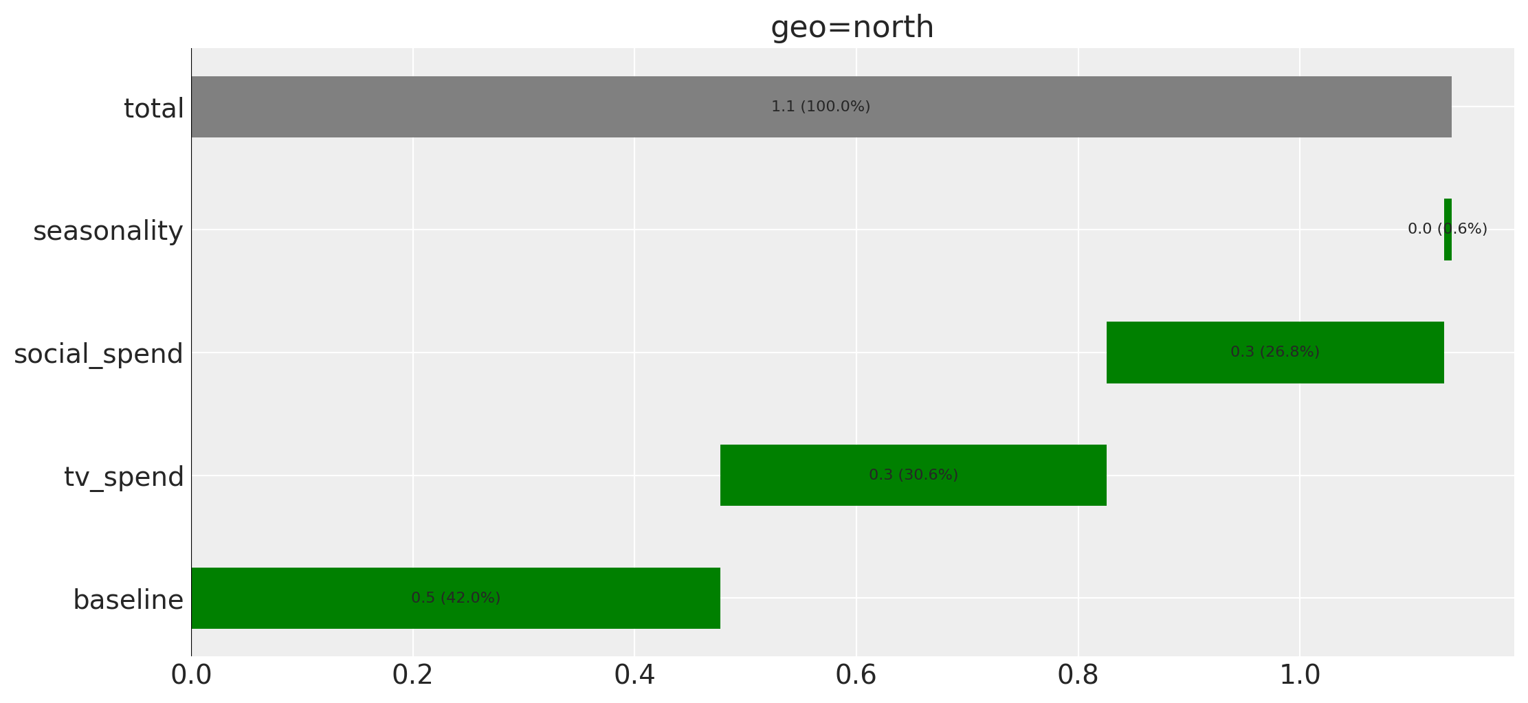
The channels bars are the direct paths only, and the mediated contribution is not redistributed into the baseline either: it is simply absent. The bars do not add up to the target:
scale = funnel.idata.constant_data["target_scale"]
post = funnel.idata.posterior
components = {
    "intercept": post["intercept_contribution"] * scale,
    "channels (direct)": post["channel_contribution_original_scale"].sum("channel"),
    "seasonality": post["yearly_seasonality_contribution"] * scale,
}
# Bars are rounded for display and summed after rounding, so the printed column
# adds up exactly.
bars = {
    name: round(float(da.sel(geo="north").mean()), 3) for name, da in components.items()
}
mediated = float(
    post["funnel_effect_contribution_original_scale"].sel(geo="north").mean()
)

two_dp_rows = ["mediated, missing from the bars", "observed target mean"]
waterfall_summary = pd.DataFrame(
    {
        "value": [
            *bars.values(),
            sum(bars.values()),
            mediated,
            float(data["y"].sel(geo="north").mean()),
        ]
    },
    index=[*bars, "sum of the waterfall bars", *two_dp_rows],
)
waterfall_summary.style.format("{:.3f}").format(
    "{:.2f}", subset=pd.IndexSlice[two_dp_rows, :]
).set_caption("Waterfall completion (geo=north, original scale)")
| value | |
|---|---|
| intercept | 0.477 |
| channels (direct) | 0.652 |
| seasonality | 0.007 |
| sum of the waterfall bars | 1.136 |
| mediated, missing from the bars | 0.61 |
| observed target mean | 1.74 |
How much of that mediated term is the channels’ due? The two tables below come from the generative model (north only, like every number above), so they are like-for-like with each other, and not with the posterior figure above.
north = geos.index("north")

pd.DataFrame(
    {
        "target units": [
            float(indirect_raw[:, north].mean()),
            float(indirect_both[:, north].mean()),
        ]
    },
    index=["true mediated term (north)", "of which the channels created"],
).style.format("{:.2f}")
| target units | |
|---|---|
| true mediated term (north) | 0.79 |
| of which the channels created | 0.40 |
mstar_parts = {
    "demand baseline": float(true["funnel_baseline"][north]),
    "category demand (gamma C)": float(
        true["funnel_gamma"][north] * category_demand[:, north].mean()
    ),
    "lf budget (lambda B)": float(
        true["funnel_lambda"][north] * lf_budget[:, north].mean()
    ),
}
mstar_mean = float(data["lf_spend_true"].sel(geo="north").mean())
mstar_parts["demand the channels created"] = mstar_mean - sum(mstar_parts.values())

pd.DataFrame(
    {
        "value (demand units)": list(mstar_parts.values()),
        "share of M*": [v / mstar_mean for v in mstar_parts.values()],
    },
    index=list(mstar_parts),
).style.format({"value (demand units)": "{:.3f}", "share of M*": "{:.1%}"}).set_caption(
    "Mean structural lower-funnel spend M* (north)"
)
| value (demand units) | share of M* | |
|---|---|---|
| demand baseline | 0.200 | 14.9% |
| category demand (gamma C) | 0.171 | 12.7% |
| lf budget (lambda B) | 0.164 | 12.2% |
| demand the channels created | 0.811 | 60.2% |
More than a third of the target is unaccounted for. Be precise about whose it is. The missing 0.61 is the entire mediated term, and lower-funnel spend is built from four things: the demand baseline, the category-demand contribution \(\gamma C\), the exogenous lower-funnel budget \(\lambda B\), and the demand the channels created. Only the last is media’s due.
Compare like with like when sizing it. The 0.61 is a posterior quantity, while the two figures in the mediated-term table are generative truth. On the true model the channels created 0.40 per week in north out of a mediated term of 0.79 (about half), and the demand baseline, the category index and the budget term split the rest. And the \(M^{*}\) percentages above are a third currency. They are shares of demand units, and the conversion from demand to target is concave, so the channels’ 60.2% of \(M^{*}\) is not their share of the missing 0.61. The joint indirect effect is.
A reader taking these bars as an attribution would therefore be wrong twice over: under-crediting both channels by their mediated contributions, and dropping the demand baseline, the category index and the budget term altogether. Between them, those three are the rest of the missing mass.
This is a boundary to know rather than a bug to route around. The DAG lives in your create_effect code, and only you can tell the library that a particular additive term means “demand this channel created”. Nearly everything causal in this notebook came from post-processing the posterior. The one built-in that follows the funnel (the incrementality module, via the effect’s opt-in) answers the per-channel spend counterfactual, not this attribution question.
Funnel-aware budget optimization#
Everything so far has been about measurement. The reason to measure is to decide, and the decision an MMM is most often asked to inform is where the money should go. This section puts the fitted funnel model through BudgetOptimizer, in-sample. We optimize the weekly allocation across the six geo \(\times\) channel cells at a fixed total. We turn the optimum into per-cell multipliers and re-weight the historical spend. Then we score the original and the re-weighted plans with the posterior and against the known truth. Three things make the exercise funnel-aware. Each is worth stating precisely, because each is a place where a funnel model can silently be optimized as if it were an ordinary one.
The intervention reaches the effect. Because the FunnelEffect reads mmm.channel_data_scaled, the optimizer’s candidate budgets move the mediated path too. Latent demand, lower-funnel spend and the conversion term are recomputed for every candidate plan, from the same graph the model was fitted with. An effect that read only its own pm.Data variables would be blind to the budgets, and the optimizer would price the media as if they created nothing downstream. The caveats at the end state the requirements this rests on.
The objective is a choice. The default response_variable, total_media_contribution_original_scale, is built from channel_contribution alone and scores the direct path. A model with mu_effects also registers total_response_original_scale: the total mean response on the original scale, summed over dates and geos, which includes the mediated term. Everything else in it (the intercept, the seasonality) does not depend on the budgets. Under the mean utility its argmax is therefore the argmax of the direct plus mediated response, and that is the objective for a funnel model. (A risk-adjusted utility would also see the baseline’s variance and should prefer a contribution variable.) We run both objectives on the same posterior, the default as a control for what pricing the mediated path changes.
The window is the training window. We optimize over the training dates themselves, so the plans can be scored against the posterior and the known truth on exactly the data the model was fitted to. create_optimization_model() fills in everything the effect needs over that window: category_demand, lf_budget and the two proxies hold exactly the values the posterior was fitted to. We pick the end date such that the window plus the model’s effective carry-over (effective_carryover_lags()) is exactly the training range. Two conventions round this out. total_budget and the optimizer’s decision variables are weekly levels per cell; the sum constraint holds on per-period budgets. And rather than spreading each cell’s weekly budget uniformly over the window, we pass budget_distribution_over_period equal to each cell’s historical spend pattern. The plan the optimizer scores is then literally “multiplier times history”: the same object we later re-weight and evaluate. Bounds are \(\pm 50\%\) around each cell’s historical weekly mean. The window’s tail carries a truncated carry-over, so what we find is an in-sample optimum, not a steady-state one.
carryover_lags = funnel.effective_carryover_lags()  # l_max + the effect's declared lags
opt_model = funnel.create_optimization_model(
    start_date=date_range[0], end_date=date_range[-(carryover_lags + 1)]
)
# Window plus effective carry-over is exactly the training range;
# create_optimization_model restores the observed values of every variable the
# effects read over those dates.
if len(opt_model.coords["date"]) != n_dates:
    raise ValueError("the optimization window does not match the training dates")
The budget is the historical one: each cell’s mean weekly spend, summed over the six cells, with the historical week-by-week pattern kept fixed. The optimizer redistributes across cells, not across time.
spend_hist = data[channels].to_array("channel").transpose("date", "geo", "channel")
mean_plan = spend_hist.mean("date")
total_budget = float(mean_plan.sum())
budget_pattern = spend_hist / spend_hist.sum("date")
budget_bounds = xr.concat(
    [0.5 * mean_plan, 1.5 * mean_plan],
    dim=pd.Index(["lower", "upper"], name="bound"),
)

print(f"total weekly budget: {total_budget:.3f}")
mean_plan.to_pandas().style.format("{:.3f}").set_caption(
    "Historical mean weekly spend per geo x channel"
)
total weekly budget: 4.316
| channel | tv_spend | social_spend |
|---|---|---|
| geo | ||
| north | 1.205 | 0.786 |
| south | 0.844 | 0.561 |
| west | 0.555 | 0.365 |
def make_optimizer(response_variable: str) -> BudgetOptimizer:
    """Build a BudgetOptimizer on the funnel model for one objective.

    Parameters
    ----------
    response_variable : str
        Name of the scalar model variable to maximise on average over the posterior.

    Returns
    -------
    BudgetOptimizer
        Optimizer over the six geo x channel weekly budgets, with the historical
        spend pattern fixed over the training window.
    """
    # Default compile mode; the caveats name Mode(linker="cvm") as the fallback
    # for an effect whose graph trips the default backend.
    return BudgetOptimizer(
        model=opt_model,
        idata=funnel.idata,
        num_periods=n_dates,
        adstock_periods=0,
        response_variable=response_variable,
        budget_distribution_over_period=budget_pattern,
    )


direct_label, funnel_label = "direct-only objective", "funnel-aware objective"
optimizers = {
    direct_label: make_optimizer("total_media_contribution_original_scale"),
    funnel_label: make_optimizer("total_response_original_scale"),
}
Before optimizing, we check that the optimizer really sees the funnel, by evaluating and differentiating, through its public API, the responses it works with. Three identities must hold. First, at the historical plan the direct, the mediated and the total response each equal the in-sample posterior mean of the corresponding variable. That proves the fixed pattern reproduces history and the effect is evaluated with the training data. Second, the marginal of the mediated response with respect to every cell’s weekly spend is positive: the mediated path moves under the intervention, cell by cell. Third, the marginal of the total response is the marginal of the direct plus the marginal of the mediated term: the objective is direct plus mediated plus a budget-independent baseline. Only once all three hold do we let the optimizers move money.
post = funnel.idata.posterior
response_vars = {
    "direct": "channel_contribution_original_scale",
    "mediated": "funnel_effect_contribution_original_scale",
    "total": "total_response_original_scale",
}
optimizer = optimizers[funnel_label]
flat = optimizer.optimization_variables.flat


def mean_over_posterior(name: str):
    """Sum a response graph over its dims and average it over the posterior draws."""
    response = optimizer.extract_response_distribution(name)
    reduce_dims = [dim for dim in response.dims if dim != "sample"]
    if reduce_dims:
        response = response.sum(dim=reduce_dims)
    return response.mean(dim="sample")


def gradient_of(name: str):
    """Exact gradient of a response's posterior mean with respect to the decision vector.

    xtensor Ops have no gradients yet, so the graph is lowered to plain tensor
    Ops first, as the optimizer does for its own objective.
    """
    scalar = rewrite_graph(
        mean_over_posterior(name).values,
        include=("lower_xtensor", "canonicalize", "stabilize"),
    )
    return pytensor.grad(scalar, flat)


# The gradient of the structural lower-funnel spend is the demand a cell creates
# per unit of its spend (the coefficient on D in M* is one); it splits the
# mediated marginal into demand created and demand converted further below.
gradient_vars = {**response_vars, "induced": "funnel_lf_spend"}
evaluate = pytensor.function(
    [flat], [mean_over_posterior(name) for name in response_vars.values()]
)
gradients = pytensor.function(
    [flat], [gradient_of(name) for name in gradient_vars.values()]
)


def response_at(x: np.ndarray) -> pd.Series:
    """Posterior-mean direct, mediated and total response of a flat weekly plan."""
    return pd.Series(
        [float(value) for value in evaluate(x)], index=list(response_vars), dtype=float
    )


x0 = optimizer.optimization_variables.pack(mean_plan)
at_history = response_at(x0)
in_sample = pd.Series(
    {
        "direct": post[response_vars["direct"]].sum(("date", "geo", "channel")).mean(),
        "mediated": post[response_vars["mediated"]].sum(("date", "geo")).mean(),
        "total": post[response_vars["total"]].mean(),
    },
    dtype=float,
)
np.testing.assert_allclose(at_history, in_sample, rtol=1e-6)

# The same cell labels serve every per-cell table below; everything is indexed
# by label, never by position in the flat vector.
mask = optimizer.budgets_to_optimize
cell_index = list(itertools.product(mask["geo"].values, mask["channel"].values))
cell_labels = [f"{geo}, {channel}" for geo, channel in cell_index]


def marginals_at(x: np.ndarray) -> pd.DataFrame:
    """Marginal response per unit of weekly spend in each cell, summed over the window.

    Parameters
    ----------
    x : np.ndarray
        Flat weekly plan, in the optimizer's decision-vector layout.

    Returns
    -------
    pd.DataFrame
        One row per geo x channel cell; the direct, mediated and total response
        and the induced lower-funnel spend, differentiated with respect to that
        cell's weekly spend.
    """
    columns = {}
    for part, gradient in zip(gradient_vars, gradients(x), strict=True):
        labelled = optimizer.optimization_variables.unpack(gradient)[
            optimizer.channel_data_var
        ]
        columns[part] = [
            float(labelled.sel(geo=geo, channel=channel)) for geo, channel in cell_index
        ]
    return pd.DataFrame(columns, index=cell_labels)


marginals = marginals_at(x0)

if not (marginals["mediated"] > 0).all():
    raise RuntimeError("the mediated term does not increase with every cell's spend")

np.testing.assert_allclose(
    marginals["total"], marginals["direct"] + marginals["mediated"], rtol=1e-6
)

if not all(opt.budgets_to_optimize.all() for opt in optimizers.values()):
    raise RuntimeError("some geo x channel cell was left out of the optimization")

np.testing.assert_array_equal(
    x0, optimizers[direct_label].optimization_variables.pack(mean_plan)
)

print(f"direct response at the historical plan:   {at_history['direct']:.2f}")
print(f"mediated response at the historical plan: {at_history['mediated']:.2f}")
print(
    f"total response at the historical plan:    {at_history['total']:.2f}"
    " (the funnel-aware objective; it includes the baseline)"
)
direct response at the historical plan:   222.56
mediated response at the historical plan: 193.25
total response at the historical plan:    536.20 (the funnel-aware objective; it includes the baseline)
The marginals are the quantity the decision turns on: the marginal response of each cell per extra unit of weekly spend, and how it splits between the direct and the mediated path. An interior optimum equalises this marginal across cells. The ordering of the total column therefore says where the funnel-aware optimizer moves money. The ordering of the direct column says where the default objective moves it. The share column is what the default objective gets wrong per cell. Because the data are synthetic, the same marginals can be computed on the generative model, clamped to the true parameters as in the true decomposition above, via central differences of \(\pm 0.5\%\) around the historical plan. Reading the two halves of the table side by side is the check that the optimizer sees the funnel with roughly the right slope, cell by cell, and not merely that it sees something.
def true_response_parts(multiplier: xr.DataArray) -> pd.Series:
    """Direct and media-created mediated response, and lower-funnel spend, of a plan on the truth.

    Parameters
    ----------
    multiplier : xr.DataArray
        Per-cell multipliers with dims ``("geo", "channel")`` applied to the
        historical media plan.

    Returns
    -------
    pd.Series
        ``direct`` and ``mediated`` response summed over the window (the mediated
        part net of the both-channels-off pass), and the structural lower-funnel
        spend ``lf_spend`` the plan induces, all on the clamped generative model.
    """
    media = (
        media_raw
        * multiplier.sel(geo=geos, channel=channels)
        .transpose("geo", "channel")
        .to_numpy()[None]
    )
    names = [
        "channel_contribution_original_scale",
        "funnel_effect_contribution_original_scale",
        "funnel_lf_spend",
    ]
    # Every parameter is clamped, so this is one deterministic forward pass;
    # the historical media are restored whatever happens in between.
    with gen.model:
        try:
            pm.set_data({"channel_data": media})
            values = pm.draw([gen.model[name] for name in names])
        finally:
            pm.set_data({"channel_data": media_raw})
    draw = {
        name: xr.DataArray(value, dims=gen.model.named_vars_to_dims[name])
        for name, value in zip(names, values, strict=True)
    }
    mediated = (
        draw["funnel_effect_contribution_original_scale"]
        .transpose("date", "geo")
        .to_numpy()
        - cf_gen["both"]["funnel_effect_contribution_original_scale"]
    )
    return pd.Series(
        {
            "direct": float(draw["channel_contribution_original_scale"].sum()),
            "mediated": float(mediated.sum()),
            "lf_spend": float(draw["funnel_lf_spend"].sum()),
        },
        dtype=float,
    )


true_at_history = true_response_parts(xr.ones_like(mean_plan))

# Central differences of +/-0.5% around the historical plan, per unit of the
# cell's mean weekly spend, indexed by the same labels as the posterior gradients.
true_marginal_rows = {}
for label, (geo, channel) in zip(cell_labels, cell_index, strict=True):
    up, down = xr.ones_like(mean_plan), xr.ones_like(mean_plan)
    up.loc[{"geo": geo, "channel": channel}] = 1.005
    down.loc[{"geo": geo, "channel": channel}] = 0.995
    per_unit = 0.01 * float(mean_plan.sel(geo=geo, channel=channel))
    true_marginal_rows[label] = (
        true_response_parts(up) - true_response_parts(down)
    ) / per_unit

true_marginals = pd.DataFrame(true_marginal_rows).T.rename(
    columns={"lf_spend": "induced"}
)
true_marginals["total"] = true_marginals["direct"] + true_marginals["mediated"]
np.testing.assert_allclose(gen.model["channel_data"].get_value(), media_raw)

marginal_table = pd.concat(
    {
        "posterior": marginals[["direct", "mediated", "total"]].assign(
            **{
                "share the default objective sees": marginals["direct"]
                / marginals["total"]
            }
        ),
        "truth": true_marginals[["direct", "mediated", "total"]],
    },
    axis=1,
)
marginal_table.style.format("{:.1f}").format(
    "{:.0%}", subset=[("posterior", "share the default objective sees")]
).set_caption(
    "Marginal response per extra unit of weekly spend in a cell, summed over the window"
    " (posterior: exact gradient; truth: central differences)"
)
| posterior | truth | ||||||
|---|---|---|---|---|---|---|---|
| direct | mediated | total | share the default objective sees | direct | mediated | total | |
| north, tv_spend | 24.5 | 9.6 | 34.2 | 72% | 23.2 | 11.1 | 34.3 |
| north, social_spend | 21.2 | 10.3 | 31.5 | 67% | 20.5 | 12.9 | 33.5 |
| south, tv_spend | 24.9 | 19.8 | 44.7 | 56% | 27.8 | 16.0 | 43.8 |
| south, social_spend | 36.5 | 16.4 | 52.8 | 69% | 26.0 | 17.4 | 43.4 |
| west, tv_spend | 37.9 | 17.7 | 55.6 | 68% | 32.5 | 19.6 | 52.1 |
| west, social_spend | 30.5 | 23.1 | 53.6 | 57% | 31.9 | 20.4 | 52.4 |
Both runs start from the historical plan and share the bounds and the total. Each optimizer maximises its own objective. The funnel-aware optimum therefore cannot score below the direct-only optimum on the total response, nor the direct-only optimum below the funnel-aware one on the direct response. Both optima also come out strictly interior to the \(\pm 50\%\) box, so the plans can be read as marginal-equalizing rather than bound-driven.
minimize_kwargs = {"options": {"ftol": 1e-8, "maxiter": 2_000}}

allocations = {}
for label, opt in optimizers.items():
    result = opt.allocate_budget(
        total_budget=total_budget,
        budget_bounds=budget_bounds,
        x0=mean_plan,
        minimize_kwargs=minimize_kwargs,
    )
    if not result.scipy_result.success:
        raise RuntimeError(f"{label}: {result.scipy_result.message}")
    np.testing.assert_allclose(result.budgets.sum(), total_budget, rtol=1e-6)
    allocations[label] = result
    print(
        f"{label}: {result.scipy_result.message} ({result.scipy_result.nit} iterations)"
    )

multipliers = xr.concat(
    [allocations[label].budgets / mean_plan for label in allocations],
    dim=pd.Index(list(allocations), name="plan"),
)
# Strictly interior: every multiplier at least 2% of the box's width away from
# the bounds, derived from the bounds actually in force.
bound_ratio = budget_bounds / mean_plan
lower_ratio = float(bound_ratio.sel(bound="lower").max())
upper_ratio = float(bound_ratio.sel(bound="upper").min())
margin = 0.02 * (upper_ratio - lower_ratio)
if (
    float(multipliers.min()) < lower_ratio + margin
    or float(multipliers.max()) > upper_ratio - margin
):
    raise RuntimeError("an optimal multiplier sits at the budget bounds")

# Each optimizer wins on its own objective, up to a slack tied to the solver's ftol.
at_optimum = {
    label: response_at(allocations[label].scipy_result.x) for label in allocations
}
ftol = minimize_kwargs["options"]["ftol"]
for winner, loser, part in [
    (funnel_label, direct_label, "total"),
    (direct_label, funnel_label, "direct"),
]:
    slack = 10 * ftol * max(abs(at_optimum[winner][part]), 1.0)
    if at_optimum[winner][part] < at_optimum[loser][part] - slack:
        raise RuntimeError(f"the {winner} optimum loses on its own objective")

comparison = pd.DataFrame(
    {
        label: multipliers.sel(plan=label).stack(cell=("geo", "channel")).to_pandas()
        for label in allocations
    }
)
comparison.index = [f"{geo}, {channel}" for geo, channel in comparison.index]
comparison["difference (funnel - direct)"] = (
    comparison[funnel_label] - comparison[direct_label]
)
comparison["same direction"] = np.sign(comparison[funnel_label] - 1) == np.sign(
    comparison[direct_label] - 1
)
comparison.style.format("{:.3f}", subset=comparison.columns[:3]).set_caption(
    "Optimal weekly spend as a multiple of the historical mean"
)
direct-only objective: Optimization terminated successfully (11 iterations)
funnel-aware objective: Optimization terminated successfully (11 iterations)
| direct-only objective | funnel-aware objective | difference (funnel - direct) | same direction | |
|---|---|---|---|---|
| north, tv_spend | 0.904 | 0.805 | -0.099 | True |
| north, social_spend | 0.870 | 0.834 | -0.036 | True |
| south, tv_spend | 0.921 | 1.074 | 0.153 | False |
| south, social_spend | 1.178 | 1.169 | -0.009 | True |
| west, tv_spend | 1.288 | 1.258 | -0.029 | True |
| west, social_spend | 1.068 | 1.177 | 0.109 | True |
The two objectives agree on the direction of most moves and disagree on some, and the marginal table above says why. A cell whose direct marginal is modest can still carry a large mediated marginal, and pricing that path is what changes its recommendation. The figure shows the historical mean and both optima side by side. The subsection after it reads every move, and in particular the north and south TV cells, off the marginals.
allocation_table = pd.concat(
    {
        "historical mean": mean_plan.stack(cell=("geo", "channel")).to_pandas(),
        **{
            label: allocations[label].budgets.stack(cell=("geo", "channel")).to_pandas()
            for label in allocations
        },
    },
    axis=1,
)
allocation_table.index = [
    f"{geo}, {channel}" for geo, channel in allocation_table.index
]

fig, ax = plt.subplots(figsize=(11, 6))
allocation_table.iloc[::-1].plot.barh(color=["gray", "C0", "C1"], ax=ax)
ax.set(xlabel="weekly spend", ylabel="")
ax.legend(loc="lower right")
ax.set_title(
    "Weekly budget per cell: historical vs optimized", fontsize=15, fontweight="bold"
)
fig.set_layout_engine("tight")
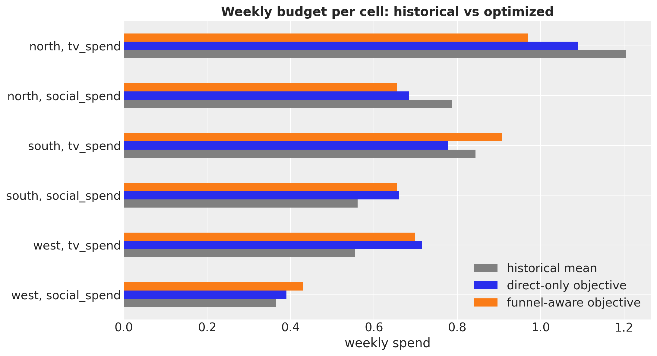
Why the plans differ where they do#
At an interior optimum with one budget constraint, the optimizer equalises, across the cells it can move money between, the marginal it sees per unit of weekly spend. That common value is the multiplier on the budget constraint, and the cell below reads it off both optima. The default objective equalises the direct marginal, the funnel-aware objective the total one. Two consequences follow. First, whether a cell is cut or grown is decided by where its marginal at the historical plan sits relative to that level. With diminishing returns, a marginal below the level rises only if the cell is cut, and one above it falls only if the cell grows. (The shared demand pool couples the two channels of a geo, so this reads one cell at a time rather than stating an identity; the six directions in the comparison table above are the ones it predicts.) Second, how far a cell moves depends on its curvature as well. The multipliers that can be compared cleanly are therefore those of cells that share their curvature parameters and their position on the response curve. The north and south TV cells are such a pair. TV’s carry-over and saturation parameters are pooled across geos, and the two cells spend at nearly the same point of the scaled curve: a mean week of 0.46 and 0.47 of each cell’s maximum.
optimum_marginals = {
    label: marginals_at(allocations[label].scipy_result.x) for label in allocations
}
# The equalisation is checked at a relative 1e-2, the sharpness a first-order
# condition supports at the solver tolerance used above.
equalisation_rtol = 1e-2
equalised = {}
for label, part in [(direct_label, "direct"), (funnel_label, "total")]:
    values = optimum_marginals[label][part]
    spread = float(values.max() - values.min()) / float(values.mean())
    if spread > equalisation_rtol:
        raise RuntimeError(f"{label}: the {part} marginals are not equalised")
    equalised[label] = float(values.mean())

marginals_by_plan = pd.concat(
    {
        "historical plan": marginals[["direct", "mediated", "total"]],
        **{
            label: pd.concat(
                [
                    comparison.loc[cell_labels, label].rename("multiplier"),
                    optimum_marginals[label][["direct", "total"]],
                ],
                axis=1,
            )
            for label in allocations
        },
    },
    axis=1,
)
marginals_by_plan.style.format("{:.1f}").format(
    "{:.3f}", subset=[(label, "multiplier") for label in allocations]
).set_caption(
    "Marginal response per unit of weekly spend at the historical plan and at each"
    f" optimum; the direct-only optimum equalises the direct marginal at"
    f" {equalised[direct_label]:.1f}, the funnel-aware optimum the total marginal at"
    f" {equalised[funnel_label]:.1f}"
)
| historical plan | direct-only objective | funnel-aware objective | |||||||
|---|---|---|---|---|---|---|---|---|---|
| direct | mediated | total | multiplier | direct | total | multiplier | direct | total | |
| north, tv_spend | 24.5 | 9.6 | 34.2 | 0.904 | 26.9 | 37.6 | 0.805 | 29.6 | 41.3 |
| north, social_spend | 21.2 | 10.3 | 31.5 | 0.870 | 26.9 | 38.8 | 0.834 | 28.8 | 41.3 |
| south, tv_spend | 24.9 | 19.8 | 44.7 | 0.921 | 26.9 | 47.9 | 1.074 | 23.1 | 41.3 |
| south, social_spend | 36.5 | 16.4 | 52.8 | 1.178 | 26.9 | 41.2 | 1.169 | 27.4 | 41.3 |
| west, tv_spend | 37.9 | 17.7 | 55.6 | 1.288 | 26.9 | 40.1 | 1.258 | 27.9 | 41.3 |
| west, social_spend | 30.5 | 23.1 | 53.6 | 1.068 | 26.9 | 48.2 | 1.177 | 22.1 | 41.3 |
The figure puts the reading rule in one picture: each cell’s marginal at the historical plan, split into its direct and mediated part, against the two levels. A cell whose direct bar ends to the left of the first line is cut by the direct-only optimizer. A cell whose full bar ends to the left of the second line is cut by the funnel-aware one.
fig, ax = plt.subplots(figsize=(11, 5))
marginals.loc[cell_labels[::-1], ["direct", "mediated"]].plot.barh(
    stacked=True, color=["C0", "C1"], ax=ax
)
ax.axvline(
    equalised[direct_label],
    color="C0",
    linestyle="--",
    linewidth=2,
    label=f"direct marginal at the direct-only optimum ({equalised[direct_label]:.1f})",
)
ax.axvline(
    equalised[funnel_label],
    color="C1",
    linestyle="--",
    linewidth=2,
    label=f"total marginal at the funnel-aware optimum ({equalised[funnel_label]:.1f})",
)
ax.set(xlabel="marginal response per unit of weekly spend, summed over the window")
ax.legend(loc="upper center", bbox_to_anchor=(0.5, -0.18), ncol=2, frameon=False)
ax.set_title(
    "Marginal response per cell at the historical plan", fontsize=15, fontweight="bold"
)
fig.set_layout_engine("tight")
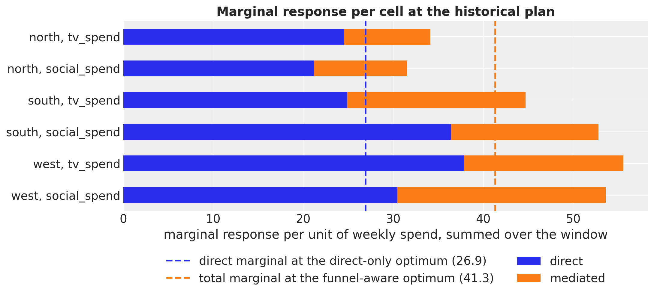
Two cells sit below both levels (north, both channels) and are cut by both objectives. Three sit above both (south, social_spend and west, both channels) and are grown by both. south, tv_spend is the one cell that straddles them, below the direct level and above the total one, which is the sign flip in the comparison table. What remains is why the mediated marginals differ as they do, and that is a question about the fit’s funnel. The mediated marginal is the product of two things. The first is the demand a unit of the cell’s spend creates over the window. (That is also the lower-funnel spend the cell induces per unit of its own spend, since \(M^{*} = D + \lambda B\) with a unit coefficient on \(D\).) The second is how much response a unit of that demand buys, which tracks the slope of the shared conversion curve at the geo’s level of structural lower-funnel spend. The first is a property of the cell, its demand-equation amplitude and its scale. The second is a property of the geo. Strictly, the second is a ratio of two window-summed marginals, so it is a demand-weighted average of that slope over the window rather than its value at a point. The two channels of a geo come out at the same number, which is what makes reading it as a property of the geo safe.
def conversion_split(table: pd.DataFrame) -> pd.DataFrame:
    """Split a mediated marginal into demand created per unit of spend and its conversion."""
    return pd.DataFrame(
        {
            "induced lower-funnel spend per unit": table["induced"],
            "response per unit of induced spend": table["mediated"] / table["induced"],
            "mediated": table["mediated"],
        }
    )


mediated_split = pd.concat(
    {
        "posterior": conversion_split(marginals),
        "truth": conversion_split(true_marginals),
    },
    axis=1,
)
lf_level = pd.DataFrame(
    {
        "posterior mean": post["funnel_lf_spend"]
        .mean(("chain", "draw", "date"))
        .to_pandas(),
        "truth": data["lf_spend_true"].mean("date").to_pandas(),
    }
)
print("structural lower-funnel spend per week, mean over the window:")
print(lf_level.round(3).to_string())

# The channel scale is each cell's maximum week of spend, so a unit of raw spend
# is a smaller step up the (pooled) response curves of a larger cell.
channel_scale = funnel.idata.constant_data["channel_scale"].transpose("geo", "channel")
spend_position = pd.concat(
    {
        "channel scale (max weekly spend)": channel_scale.to_pandas(),
        "mean week as a share of the scale": (mean_plan / channel_scale).to_pandas(),
    },
    axis=1,
)
print("\nwhere each cell's mean week sits on its own scale:")
print(spend_position.round(3).to_string())
mediated_split.style.format("{:.1f}").format(
    "{:.2f}",
    subset=[
        (half, "response per unit of induced spend") for half in ("posterior", "truth")
    ],
).set_caption(
    "The mediated marginal as demand created times demand converted, per cell"
)
structural lower-funnel spend per week, mean over the window:
       posterior mean  truth
geo
north           1.344  1.347
south           1.034  1.029
west            0.781  0.777

where each cell's mean week sits on its own scale:
        channel scale (max weekly spend)              mean week as a share of the scale
channel                         tv_spend social_spend                          tv_spend social_spend
geo
north                              2.607        1.295                             0.462        0.607
south                              1.791        0.997                             0.471        0.562
west                               1.046        0.611                             0.531        0.597
| posterior | truth | |||||
|---|---|---|---|---|---|---|
| induced lower-funnel spend per unit | response per unit of induced spend | mediated | induced lower-funnel spend per unit | response per unit of induced spend | mediated | |
| north, tv_spend | 31.0 | 0.31 | 9.6 | 34.5 | 0.32 | 11.1 |
| north, social_spend | 32.7 | 0.32 | 10.3 | 38.3 | 0.34 | 12.9 |
| south, tv_spend | 46.6 | 0.43 | 19.8 | 41.6 | 0.38 | 16.0 |
| south, social_spend | 38.2 | 0.43 | 16.4 | 44.1 | 0.39 | 17.4 |
| west, tv_spend | 48.6 | 0.36 | 17.7 | 50.7 | 0.39 | 19.6 |
| west, social_spend | 63.5 | 0.36 | 23.1 | 52.2 | 0.39 | 20.4 |
Read the north and south TV cells off these tables. The direct-only objective sees twins: a direct marginal of 24.5 in north against 24.9 in south per unit of weekly spend. Both sit below the 26.9 it equalises to, so it cuts both, and by about the same amount (0.904 and 0.921). The funnel-aware objective sees 34.2 against 44.7. north, tv_spend has the smallest mediated marginal of the six cells (9.6), its total has to climb to 41.3, and it takes the deepest cut of the plan (0.805). south, tv_spend starts above 41.3, so it grows (1.074) until its total marginal has fallen to that level. This is not a matter of taste between two objectives. On the generative truth the two cells’ total marginals are 34.3 and 43.8, as far apart as the posterior says. Their direct marginals differ more than the posterior thinks (23.2 against 27.8). The direct/mediated seesaw from the parameter-recovery section explains it: north TV’s direct amplitude runs high and its demand amplitude low, with south TV the other way round. That is what makes the two direct marginals look alike, and the direct-only objective is exposed to that split. The total marginal, which is what the funnel-aware objective needs, is pinned within about 7% in five of six cells even where the split is not.
Why south’s mediated marginal is twice north’s (19.8 against 9.6 per unit of spend; 16.0 against 11.1 in truth) then splits into the two factors. Demand created: a unit of TV spend induces 46.6 units of lower-funnel spend over the window in south and 31.0 in north (41.6 and 34.5 in truth). The demand-equation amplitudes sat_uf_beta are similar in the units the model sees (0.77 and 0.75). But the channel scale is a per-cell maximum, so a unit of raw spend is a smaller step up north’s curve: its maximum week is 2.61 against 1.79. The seesaw moves some of north TV’s mass to the direct path on top. Demand converted: a unit of induced spend buys 0.43 of response in south and 0.31 in north (0.38 and 0.32 in truth). That number is the same for both channels within a geo, because the conversion happens on the geo’s structural lower-funnel spend. north runs at the highest level of the three: 1.34 a week against 1.03 in south and 0.78 in west, in the posterior as in truth. It therefore sits furthest up the shared conversion curve sat_lf, where an extra unit of demand buys less. The posterior’s sat_lf_beta for south (1.125 against a true 0.90, covered but high) steepens south’s slope further. Both factors point the same way in the posterior and in the truth, and the posterior exaggerates both, which is why it also exaggerates the gap between the two cells’ mediated marginals.
In-sample evaluation#
We turn each optimum into per-cell multipliers, re-weight the historical spend, and score the plans with the posterior. The total spend is preserved by construction (the sum constraint holds on weekly levels and the pattern is fixed), which the assertion below confirms rather than enforces.
What to score is the one funnel-specific choice. The quantity a budget decision turns on is the media-driven response: the direct contributions plus the part of the mediated term that the media created. We follow the both-channels-off convention from the true decomposition above: the joint indirect effect, not the leave-one-out sum. We take the mediated term under a plan minus the mediated term with both channels switched off, per posterior draw, so the demand baseline, the category index and the lower-funnel budget cancel exactly. That needs one more posterior-predictive pass, with both channels at zero and the effect’s exogenous data at their training values, so the both-off pass differs from a plan only in the channel spend. Under the mean utility this yardstick and the objective have the same argmax; they differ by a per-draw constant. Both are recomputed here from the model rather than read off the optimizer. The loop closes when the optimizer’s own value at each optimum equals the posterior-predictive value of the re-weighted plan, for both objectives.
def sample_plan(X: pd.DataFrame) -> xr.Dataset:
    """Posterior-predictive contributions of the funnel model under a spend plan.

    Parameters
    ----------
    X : pd.DataFrame
        Long frame with the date, geo and upper-funnel channel columns.

    Returns
    -------
    xr.Dataset
        Direct, mediated and total response on the original scale, and the
        structural lower-funnel spend, per chain and draw.
    """
    return funnel.sample_posterior_predictive(
        X,
        var_names=[*response_vars.values(), "funnel_lf_spend"],
        combined=False,
        extend_idata=False,
        progressbar=False,
        random_seed=rng,
    )


def plan_frame(multiplier: xr.DataArray) -> pd.DataFrame:
    """Re-weight the historical spend by per-cell multipliers into a long frame."""
    return (spend_hist * multiplier).to_dataset("channel").to_dataframe().reset_index()


plan_frames = {label: plan_frame(multipliers.sel(plan=label)) for label in allocations}
for X_plan in plan_frames.values():
    np.testing.assert_allclose(
        X_plan[channels].to_numpy().sum(), float(spend_hist.sum()), rtol=1e-6
    )

X_zero = X_upper.copy()
X_zero[channels] = 0.0

pp = {label: sample_plan(X_plan) for label, X_plan in plan_frames.items()}
pp_zero = sample_plan(X_zero)
pp["historical"] = xr.Dataset(
    {var: post[var] for var in [*response_vars.values(), "funnel_lf_spend"]}
)
for samples in pp.values():
    xr.align(samples, pp_zero, join="exact")

mediated_zero = pp_zero[response_vars["mediated"]]
if float(mediated_zero.mean()) >= float(
    pp["historical"][response_vars["mediated"]].mean()
):
    raise RuntimeError("switching both channels off did not reduce the mediated term")
# The both-channels-off yardstick is the optimizer's own graph at zero spend.
np.testing.assert_allclose(
    mediated_zero.sum(("date", "geo")).mean(),
    response_at(np.zeros_like(x0))["mediated"],
    rtol=1e-6,
)


def media_response(samples: xr.Dataset) -> xr.DataArray:
    """Media-driven response per date: direct plus media-created mediated term."""
    direct = samples[response_vars["direct"]].sum(("geo", "channel"))
    mediated = (samples[response_vars["mediated"]] - mediated_zero).sum("geo")
    return direct + mediated


response = {label: media_response(samples) for label, samples in pp.items()}
response_total = {label: r.sum("date") for label, r in response.items()}
direct_total = {
    label: samples[response_vars["direct"]].sum(("date", "geo", "channel"))
    for label, samples in pp.items()
}
lf_spend_total = {
    label: samples["funnel_lf_spend"].sum(("date", "geo"))
    for label, samples in pp.items()
}

# Loop closure: each optimizer's reported optimum equals the posterior-predictive
# recomputation of its own objective under the re-weighted plan.
recomputed = {
    funnel_label: pp[funnel_label][response_vars["total"]].mean(),
    direct_label: direct_total[direct_label].mean(),
}
for label, part in [(funnel_label, "total"), (direct_label, "direct")]:
    np.testing.assert_allclose(at_optimum[label][part], recomputed[label], rtol=1e-6)
    np.testing.assert_allclose(
        -allocations[label].scipy_result.fun, at_optimum[label][part], rtol=1e-6
    )
Sampling: []
Sampling: []
Sampling: []
Because the data are synthetic we can also price each plan on the generative model, with the same helper that produced the true marginals above. One forward pass per plan gives the truth against which the posterior uplifts can be checked.
true_parts = {"historical": true_at_history}
for label in allocations:
    true_parts[label] = true_response_parts(multipliers.sel(plan=label))
np.testing.assert_allclose(gen.model["channel_data"].get_value(), media_raw)

true_response = {
    label: parts["direct"] + parts["mediated"] for label, parts in true_parts.items()
}
true_direct_hist = float(data["direct_true"].sum())
np.testing.assert_allclose(true_parts["historical"]["direct"], true_direct_hist)
The next three figures mirror the case study. First the plans themselves: the historical spend against the funnel-aware optimum, per channel and geo (solid versus dashed).
X_optimized = plan_frames[funnel_label]

fig, axes = plt.subplots(
    nrows=len(channels),
    ncols=len(geos),
    figsize=(16, 8),
    sharex=True,
    layout="constrained",
)
for row, (channel, color) in enumerate(zip(channels, ["C0", "C1"], strict=True)):
    for col, geo in enumerate(geos):
        ax = axes[row, col]
        original = X_upper.query("geo == @geo")
        optimized = X_optimized.query("geo == @geo")
        ax.plot(
            original["date"],
            original[channel],
            color=color,
            alpha=0.5,
            label="original",
        )
        ax.plot(
            optimized["date"],
            optimized[channel],
            color=color,
            linestyle="--",
            label=f"optimized (x{float(multipliers.sel(plan=funnel_label, geo=geo, channel=channel)):.2f})",
        )
        ax.set_title(f"{channel}, {geo}")
        ax.legend(loc="upper left", fontsize=9)
axes[-1, 0].set_xlabel("date")
fig.suptitle(
    "Original vs Optimized Budget Allocation (training data)",
    fontsize=16,
    fontweight="bold",
)
fig.autofmt_xdate()
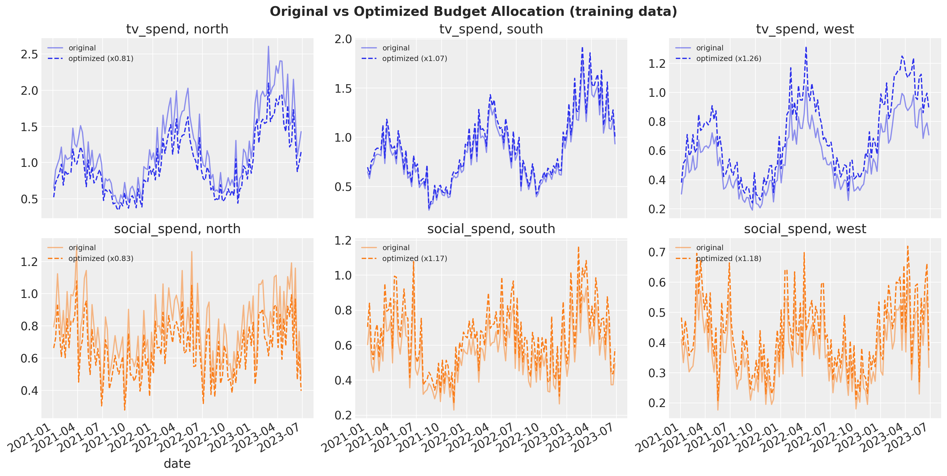
Then the media-driven response over time under the original and the funnel-aware optimized plan, summed over geos and channels, with 94% HDIs. The two bands overlap heavily: the reallocation is a modest tilt of a plan that was already close to the posterior optimum within the \(\pm 50\%\) box, not a rewrite of it.
fig, ax = plt.subplots(figsize=(13, 6))
for label, color in [("historical", "C0"), (funnel_label, "C1")]:
    lo, hi = hdi_bounds(response[label])
    ax.fill_between(date_range, lo, hi, color=color, alpha=0.3)
    ax.plot(
        date_range,
        response[label].mean(("chain", "draw")),
        color=color,
        label="original plan"
        if label == "historical"
        else "optimized plan (funnel-aware)",
    )
ax.legend(loc="upper left")
ax.set(ylabel="media-driven response (all geos, both channels)")
ax.set_title(
    "Original vs Optimized Budget Allocation (training data)",
    fontsize=16,
    fontweight="bold",
)
fig.autofmt_xdate()
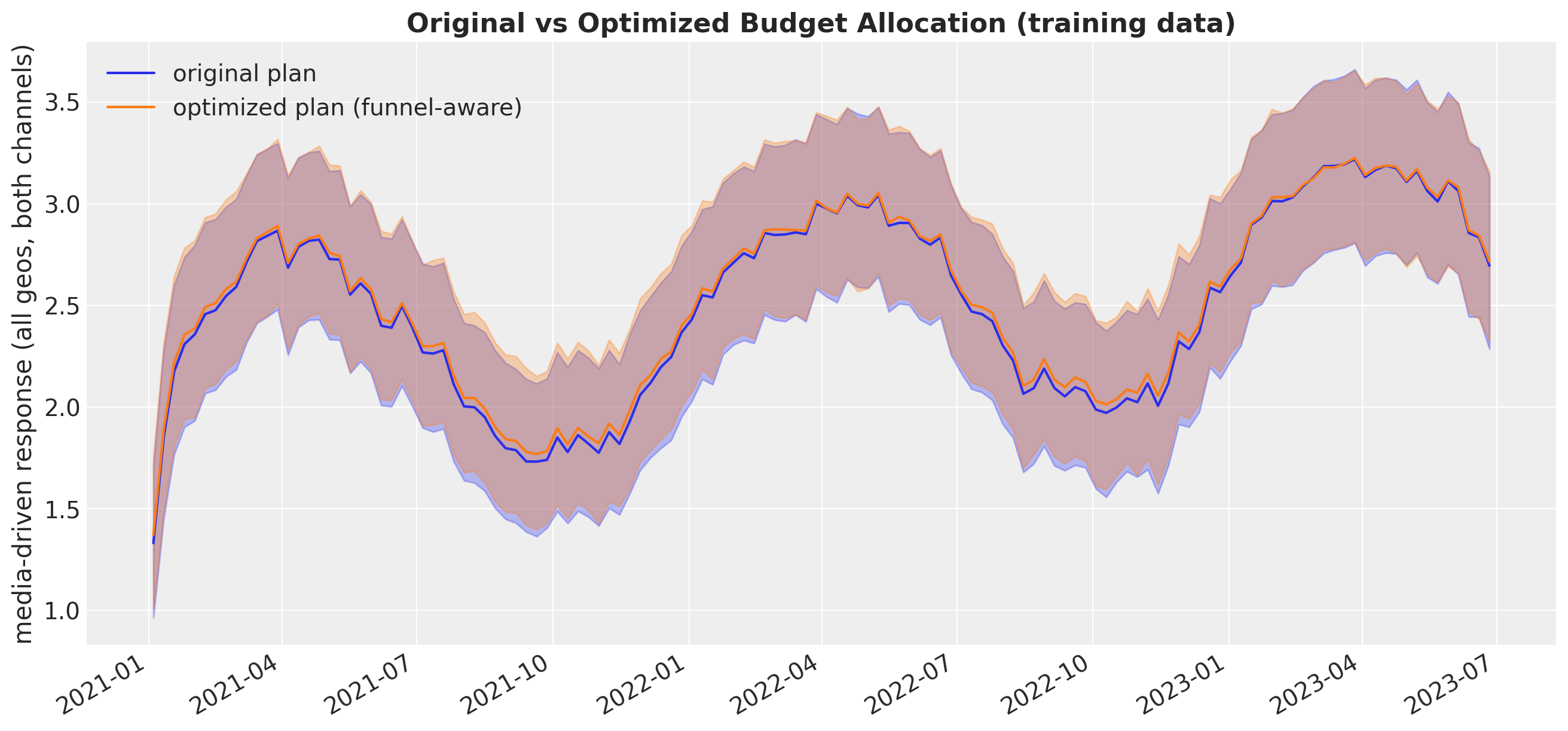
Finally the uplift, as a posterior distribution of the ratio of media-driven response under each optimized plan to that under the historical plan, with the true uplift from the generative model as a dashed line. The direct-only plan is scored with the same funnel-aware yardstick, so the two panels compare like with like. The tables add three things: what the direct-only optimizer itself believes it gained (its own objective), the absolute uplifts with their true direct and mediated parts, and the lower-funnel spend each plan induces. One convention to name: every uplift here, the self-assessed row included, is the mean of the per-draw ratios. (The optimizer’s internal objective is a posterior mean, so its reported optimum is not itself a row of these tables.)
uplift = xr.Dataset(
    {
        label: response_total[label] / response_total["historical"] - 1
        for label in allocations
    }
)
true_uplift = {
    label: true_response[label] / true_response["historical"] - 1
    for label in allocations
}

pc = azp.plot_dist(
    uplift,
    ci_kind="hdi",
    ci_prob=0.94,
    col_wrap=1,
    figure_kwargs={"figsize": (10, 9), "sharex": True},
)
fig = pc.viz["figure"].item()
xlim = (float(uplift.to_array().min()), float(uplift.to_array().max()))
for label in allocations:
    ax = pc.viz["plot"][label].item()
    ax.axvline(0, color="C3", linestyle=":", linewidth=2, label="no change")
    ax.axvline(
        true_uplift[label],
        color="black",
        linestyle="--",
        linewidth=2,
        label="true uplift",
    )
    ax.set_xlim(xlim)
    ax.xaxis.set_major_formatter(plt.matplotlib.ticker.PercentFormatter(xmax=1))
    ax.set_title(f"{label}: plan re-weighted by its optimum")
    ax.legend(loc="upper right")
fig.suptitle(
    "Uplift in media-driven response after optimization", fontsize=18, fontweight="bold"
);
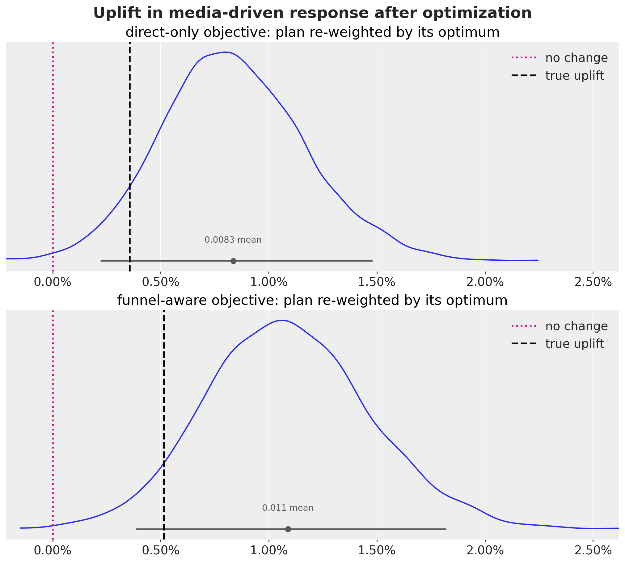
def summarise(da: xr.DataArray) -> tuple[float, float, float]:
    """Return the posterior mean and 94% HDI bounds of a scalar posterior quantity."""
    lo, hi = hdi_bounds(da)
    return float(da.mean()), float(lo), float(hi)


rows = {}
for label in allocations:
    mean, lo, hi = summarise(uplift[label])
    rows[label] = {
        "posterior mean uplift": mean,
        "94% HDI lower": lo,
        "94% HDI upper": hi,
        "true uplift": true_uplift[label],
    }
rows[direct_label]["self-assessed uplift (direct objective)"] = float(
    (direct_total[direct_label] / direct_total["historical"] - 1).mean()
)
uplift_table = pd.DataFrame(rows).T
uplift_table.style.format("{:+.2%}", na_rep="").set_caption(
    "Uplift in media-driven response versus the historical plan"
)
| posterior mean uplift | 94% HDI lower | 94% HDI upper | true uplift | self-assessed uplift (direct objective) | |
|---|---|---|---|---|---|
| direct-only objective | +0.83% | +0.22% | +1.48% | +0.36% | +0.84% |
| funnel-aware objective | +1.09% | +0.39% | +1.82% | +0.51% |
parts_rows = {}
for label in allocations:
    delta_true = true_parts[label] - true_parts["historical"]
    parts_rows[label] = {
        "absolute uplift (posterior mean)": float(
            (response_total[label] - response_total["historical"]).mean()
        ),
        "true absolute uplift": delta_true["direct"] + delta_true["mediated"],
        "true direct part": delta_true["direct"],
        "true mediated part": delta_true["mediated"],
        "induced lower-funnel spend (posterior mean)": float(
            (lf_spend_total[label] / lf_spend_total["historical"] - 1).mean()
        ),
        "induced lower-funnel spend (true)": (
            true_parts[label]["lf_spend"] / true_parts["historical"]["lf_spend"] - 1
        ),
    }
parts_table = pd.DataFrame(parts_rows).T
parts_table.style.format("{:+.2f}").format(
    "{:+.2%}", subset=parts_table.columns[-2:]
).set_caption("What the uplift is made of, and the lower-funnel spend the plan induces")
| absolute uplift (posterior mean) | true absolute uplift | true direct part | true mediated part | induced lower-funnel spend (posterior mean) | induced lower-funnel spend (true) | |
|---|---|---|---|---|---|---|
| direct-only objective | +2.69 | +1.16 | +0.34 | +0.82 | +0.36% | +0.28% |
| funnel-aware objective | +3.51 | +1.67 | +0.55 | +1.11 | +0.93% | +0.40% |
level_table = pd.DataFrame(
    {
        "posterior mean": [
            float(direct_total["historical"].mean()),
            float(response_total["historical"].mean()),
        ],
        "true value": [true_direct_hist, true_response["historical"]],
    },
    index=["direct only (default objective)", "direct + media-created mediated"],
)
level_table.loc["share the default objective sees"] = (
    level_table.iloc[0] / level_table.iloc[1]
)
level_table.style.format("{:.1f}").format(
    "{:.1%}", subset=pd.IndexSlice[["share the default objective sees"], :]
).set_caption("Media-driven response of the historical plan, summed over the window")
| posterior mean | true value | |
|---|---|---|
| direct only (default objective) | 222.6 | 197.1 |
| direct + media-created mediated | 326.2 | 324.2 |
| share the default objective sees | 68.2% | 60.8% |
Reading the results#
Take the level first, because it is the safe claim and the one that does not depend on how far the optimizer moves. At the historical plan the default objective values the media at 222.6 (posterior mean, summed over the window) against a media-driven response of 326.2. It sees 68.2% of what the media do, and on the generative truth the share is 60.8% (197.1 of 324.2). Both are level shares under the both-channels-off convention: the mediated mass in the denominator is only what the channels created, not the demand baseline, the category index or the lower-funnel budget. The marginal table is the sharper statement, because a budget decision turns on marginals, not levels. Per unit of weekly spend, the default objective sees between 56% and 72% of a cell’s marginal response. It sees least in south, tv_spend and west, social_spend, the two cells where the mediated marginal is largest relative to the direct one. Against the truth, the posterior total marginals land within about 7% in five of six cells. The exception is south, social_spend, where the posterior over-credits the direct path (per unit of weekly spend, 36.5 against a true 26.0) and overstates the cell’s total marginal by about a fifth. So the total is pinned well at the level (326.2 against 324.2), while the direct/mediated split, at the level and at the margin, is not (222.6 against 197.1). That is the weak identification of the two paths noted in the parameter-recovery section, and the marginal table is where that split can move the decision.
Then the plans. The two objectives agree on the direction of five of six moves: out of north (both channels), into west (both) and into south, social_spend. They disagree on the sign of south, tv_spend: a cut of 8% under the default objective, an increase of 7% under the funnel-aware one. They also differ by about ten points in two other cells (west, social_spend, 1.068 against 1.177; north, tv_spend, 0.904 against 0.805). The marginal tables say why. Each optimizer equalises the marginal it sees: the direct one at 26.9 per unit of weekly spend, the total one at 41.3. south, tv_spend is the one cell that sits below the first level and above the second, because its direct marginal is the twin of north TV’s while its mediated marginal is twice as large. A unit of its spend creates half again as much demand (a smaller cell on the same pooled TV curves). And south’s lower funnel converts that demand at a steeper point of the shared conversion curve than north’s, which runs at the highest structural spend level of the three geos. Pricing that path is what turns its cut into an increase. No cell touches the \(\pm 50\%\) bounds; both optima are interior.
The uplifts are small, and that is the honest reading of a synthetic plan that was already close to the posterior optimum within the \(\pm 50\%\) box. Re-weighting the history by the funnel-aware optimum lifts the media-driven response by 1.09% (94% HDI 0.39% to 1.82%); the direct-only optimum lifts it by 0.83% (0.22% to 1.48%). On the posterior yardstick the funnel-aware plan cannot score lower than the direct-only one, since it maximises exactly that quantity up to a plan-invariant constant. The independent test is the generative truth. On this dataset the funnel-aware plan is also worth more there: +0.51% against +0.36%, or 1.67 against 1.16 target units. More of each plan’s true gain travels through the mediated path than through the direct one (1.11 of 1.67, and 0.82 of 1.16): reallocations move both paths, whichever one the optimizer was looking at. Both plans induce more lower-funnel spend than history because they create more demand (+0.40% and +0.28% in truth, +0.93% and +0.36% under the posterior). The uplift is gross of that spend, which the ROAS section prices and the optimizer does not. In relative terms, the direct-only optimizer’s own verdict on its plan (+0.84% on its direct objective) is essentially the +0.83% the funnel model attributes to that plan on the full response. Here the mediated part happens to move by a similar fraction. So the third of the response the default objective cannot see shows up as a level it never counts and as the cells it gets wrong, not as an inflated percentage.
The truth lines fall inside both 94% intervals, but in their lower halves. (The intervals are not coverage claims for a plan chosen on this posterior.) The posterior overstates each plan’s absolute gain by about a factor of two: 3.51 against 1.67 target units for the funnel-aware plan, 2.69 against 1.16 for the direct-only one. That is consistent with the optimizer’s curse: a plan chosen to maximise the posterior mean is the plan the posterior’s own errors flatter. But on one synthetic dataset it is not separable from the over-credited direct marginal in south, social_spend, a cell both plans fund, nor from extrapolation. Multipliers above one push the grown cells’ peak weeks beyond the largest spend those cells were fitted on (the channel scale is a per-cell maximum), so part of each interval is extrapolation. Everything here is in-sample and inherits the truncated carry-over at the end of the window: an in-sample optimum, not a steady-state one. And it is the same fitted model under two objectives, not what a mediator-blind model would recommend. A naive model’s direct curves absorb some of the mediated mass, so its self-assessment is a different animal from the direct-only objective studied here.
Co-optimizing the lower funnel#
Everything above treats lf_budget as given: the optimizer moves media across the six geo \(\times\) channel cells and the lower-funnel budget stays where history put it. That was a limitation of the machinery rather than a modelling choice. Lower-funnel spend is money, so the decision a planner actually faces is how to divide one pot between the upper funnel and the lower one.
spend_vars names additional monetary pm.Data nodes to co-optimize. Each is decided over its own non-date dimensions – lf_budget is (date, geo), so it becomes one budget per geo – and reports its spend to the same budget-sum constraint the media budgets answer to. It is not a lever: optimizable_vars is for quantities in their own units, a discount depth or a frequency, which deliberately sit outside that constraint. Money belongs inside it.
Two things change with the problem, and both are choices rather than defaults worth accepting silently. The pot has to widen. Comparing a media-only plan of \(B\) against a joint plan of \(B\) would ask the lower funnel to be funded out of thin air, so the joint budget is what history actually spent on both. The time profile differs. Media follows the historical weekly pattern through budget_distribution_over_period; a spend variable is spread uniformly across the window unless you supply a pattern of its own.
# The joint pot is what was actually spent on both, so the two plans are
# comparable: the optimizer chooses the split rather than being handed one.
lf_mean_weekly = data["lf_budget"].mean("date")
joint_budget = total_budget + float(lf_mean_weekly.sum())

joint_optimizer = BudgetOptimizer(
    model=opt_model,
    idata=funnel.idata,
    num_periods=n_dates,
    adstock_periods=0,
    response_variable="total_response_original_scale",
    budget_distribution_over_period=budget_pattern,
    spend_vars=["lf_budget"],
)

joint_result = joint_optimizer.allocate_budget(
    total_budget=joint_budget, minimize_kwargs=minimize_kwargs
)
if not joint_result.scipy_result.success:
    raise RuntimeError(joint_result.scipy_result.message)

# `spend_var_allocations` is the monetary subset of `optimized_vars`:
# levers live there too.
media_spend = float(joint_result.budgets.sum())
lower_funnel_spend = sum(
    float(allocation.sum())
    for allocation in joint_result.spend_var_allocations.values()
)
np.testing.assert_allclose(media_spend + lower_funnel_spend, joint_budget, rtol=1e-6)

split = pd.DataFrame(
    {
        "historical": [total_budget, float(lf_mean_weekly.sum())],
        "joint optimum": [media_spend, lower_funnel_spend],
    },
    index=pd.Index(["upper funnel (media)", "lower funnel (lf_budget)"], name="pot"),
)
split.loc["total"] = split.sum()
split.style.format("{:.3f}").set_caption(
    f"Weekly spend split, one pot of {joint_budget:.3f}"
)
The same split, per geo:
pd.concat(
    {
        "historical": lf_mean_weekly.to_pandas(),
        "joint optimum": joint_result.spend_var_allocations["lf_budget"].to_pandas(),
    },
    axis=1,
).style.format("{:.3f}").set_caption(
    "Lower-funnel weekly budget per geo: given, and decided"
)
The constraint check above is the substantive one: media and lower-funnel spend are summed together and matched against a single total. Nothing in constraints.py knows a second spend exists – the default constraint totals every decision variable that reports a monetary contribution, and a spend variable joins by being one.
Read the split with the same care as the rest of this notebook. The lower funnel converts through a saturating curve shared across geos, so where the optimum lands depends on how far up that curve the historical budget already sits; and the objective is still the total media-driven response, so the plan is gross of the lower-funnel spend it induces, exactly as it was before. What is new is only that \(B\) is now chosen rather than assumed.
Caveats and extensions#
The framework does not “see” the DAG. The funnel structure lives in the
FunnelEffectcode, and no built-in decomposition knows what is upstream of what. The incrementality module is the partial exception. An effect that opts in viaincrementality_spechas its mediated response included in the per-channel spend counterfactual, but even it does not split the mediated mass among its four sources, which is the attribution at issue here. The consequences differ by tool, and the second is the sharper trap. The data-layer decomposition behind the plot suite andmmm.summary.contributionsrecognises a fixed set of components and, under this model’s identity link, omits a customMuEffectentirely, as the waterfall above shows. (Underlink="log"it is folded into the baseline instead: absorbed rather than dropped.) The counterfactual decomposition does include each registered effect as its own labelled part. But that hands you the whole mediated mass as onefunnel_effectbar, not the channels’ causal due. Splitting the bar is the post-processing done above, and anything causal has to come from there.Pass a
Dataset, not aDataFrame. Extra columns in a DataFrame are dropped during conversion, so aDataVarMuEffectwould not find its variables. Build the model from anxarray.Dataset.fitstill takes the long frame for its bookkeeping, which is also whyfit_datacarries no funnel columns, and why asave/build_from_idataround-trip would not reconstruct this model.Pooling choices are identification choices. We pooled carryover and curvature across geos and left amplitudes free. Freeing everything per geo with ~130 weeks each will widen the posteriors considerably and can introduce divergences; hierarchical (partially pooled) priors are the natural next step.
Latent variables need an anchor. Fixing at one the coefficient on \(D\) in the lower-funnel spend equation is what gives \(D\) a scale: latent demand is expressed in units of the spend it induces. Leave that coefficient free as well as \(\kappa\) and the model is unidentified. Which relationship you anchor to is a substantive choice, because it decides what “one unit of demand” means.
The two exclusion restrictions are not equally load-bearing. The budget’s restriction (\(B\) enters the spend equation but not the search equation) is genuinely identifying. It is what separates \(\lambda B\) from \(D\). It has a testable implication, \(B \perp S\) on the raw data, which we verified both on the graph and empirically. Dropping it, or giving the budget no independent variation, merges \(\lambda\) into the demand baseline. Category demand’s restriction (\(C\) absent from the target equation) is a modelling convenience: \(C\) is observed, so a \(C \to Y\) path could be absorbed by adding it as a control column, exactly as
Naive B+does.Only one downstream variable is a cause. Lower-funnel spend belongs in the target equation; branded search does not. Getting that backwards is not a modelling nicety, it is the difference between
Naive Cand the funnel model.Graph verdicts are conditional on the graph, including the parts you almost did not draw. The d-separation table split the market driver into three strands: a seasonal basis, a growth trend, and the drivers’ shared noise. Only the first two are observed. That third strand is easy to leave out of a drawing; it came from one
LKJCholeskyCovline in the DGP. Leaving it out certifiesNaive B++as a valid total-effect estimator, which on the full graph it is not: a trend control blocks the fork it names and nothing else. A reader who believed the Fourier basis captured the entire driver would have gone further and scoredNaive Bas valid. On real data the analogous question cannot be checked against a known truth: what is the market driver, which strands of it do your regressors span, and what is left over? A genuinely latent residue (taste shifts, competitor activity) puts even the trend fix out of reach. Controlling for a measured demand index helps exactly as far as the problem is confounding. Here it repaired the trend-confounded channel and did nothing for the bias that was never materially confounded. Making the index part of a correctly specified structural equation, as the funnel model does, is what addresses the rest. The same caution applies to the drawing’s shape. It collapses time, so every verdict above is a statement about one time slice of a system whose adstocks are lagged. That reading is right for an MMM, whose control columns condition on whole series, but a confounder that acted only with a lag would need a graph that shows time.The funnel model is handed the true functional form. In this synthetic exercise the funnel model is the DGP: right response families, right pooling structure, right anchoring, right exclusion restrictions. That is the strongest possible version of the comparison, and it is also the point. The notebook’s thesis is that structure, not adjustment, is what separates the specifications, so the model given the correct structure should win, and by how much is worth knowing. On real data nobody hands you the functional form. The parameter-recovery and proxy-predictive checks above are the tools for arguing your structural equations are close enough, and misspecifying them would erode the funnel model’s advantage exactly where the naive models lose theirs.
The funnel model’s advantage mixes structure with information. It observes two likelihood series and two inputs the naive models never see, so its narrower intervals are not attributable to structure alone. The clean way to separate the two is a specification that sees the extra series without modelling the system:
Naive B++withlower_spendandsearch_volumeadded as control columns, which we leave as an exercise. Note that conditioning on either one is conditioning on a descendant of the treatment, so it answers a different causal question, which is rather the point.Distinguish a mediator from an organic path. We route the entire mediated effect through lower-funnel spend. A model with both \(M^{*} \to Y\) and a direct organic \(D \to Y\) is more realistic still. But the two differ only by \(\lambda B\) and would be weakly separated at this sample size: a good reason to add such a path only with data (or priors) that can support it.
Per-channel indirect effects are not additive. With a shared saturating mediator, leave-one-out attribution understates the joint effect, here by about 13%. Report the convention alongside the number; Mediation Analysis and (In)Direct Effects with PyMC works through the general decomposition, where the pieces that leave-one-out drops appear as explicit interaction and dependence terms.
Mind the scales. The base
MMMscales its channel and target data, but aDataVarMuEffectreads its variables unscaled. Here the data is generated in-model at roughly unit scale, so theHalfNormal(1)priors in the demand equation are sensible. On real data, scale those inputs (or the priors) yourself.Budget optimization with a custom effect has three requirements, and one thing it does not do. (1) The effect must read the model’s channel data. It is
create_effectreadingmmm.channel_data_scaledthat lets the optimizer’s intervention onchannel_datareach the mediated path. An effect that read only its ownpm.Datavariables would be untouched by it, and the optimizer would silently price the direct path alone. (2) The objective must betotal_response_original_scale, since the defaultresponse_variablecounts the direct path only.budget_optimizer()warns when it detects a mediated effect and no objective is named. ABudgetOptimizerbuilt directly on a model, as the in-sample flow above requires, cannot warn, so name it. (3) The effect’s exogenous data must cover the window, andcreate_optimization_modeltakes care of it: observed values on the dates the training data covers, zeros beyond, with the carry-over sized byeffective_carryover_lags(). In-sample that reproduces the training data exactly, as above. For a future window the zeros are a scenario choice (“no committed activity”). To plan against committed activity,pm.set_datathe effect’s variables with the values you expect before handing the model toBudgetOptimizer. A window that does not open at the start of training also needscarry_in_periods, so that the carry-in, decision and adstock periods together cover the model’s date range;budget_optimizer()sets all three itself. Lower-funnel spend can itself be a decision: name it inspend_varsand it becomes a per-geo monetary variable competing with media for one total, as Co-optimizing the lower funnel does. If a differently shaped effect trips a compile-backend limitation (a chained, sample-batched convolution can, see pymc-devs/pytensor#2360),compile_kwargs={"mode": pytensor.compile.mode.Mode(linker="cvm")}is the fallback. What the optimizer does not do: it does not count the lower-funnel spend the plan induces. \(M^{*} = D + \lambda B\) rises with the demand a plan creates, so the media-driven uplift above is gross of that spend, which the tables report next to it. What the optimizer needs is only the total media-driven response, so the attribution ambiguity of the shared saturating pool discussed above never enters it. The in-sample optimum also inherits the truncated carry-over at the end of the window: an in-sample rather than a steady-state optimum.
Natural extensions: hierarchical priors across geos, censored lower-funnel spend for budget-capped channels, more than one latent demand pool (for example separate branded and non-branded demand), and time-varying mediator baselines.
References#
The Nürnberger Versicherung case-study series from PyMC Labs, which works through the same funnel problem in a production setting:
Cracking the Funnel: How Nürnberger Quantified Cross-Channel Synergies (Part I)
Building a Funnel-Aware Bayesian Marketing Mix Model (Part II)
A PyMC-Marketing Case Study: Campaign Dynamics, Influencer Effectiveness, and Time-Slice CV (Part III)
On the graphical machinery used in What the graph already says:
Pearl, J., Glymour, M., and Jewell, N. P. (2016). Causal Inference in Statistics: A Primer. Wiley. Chapters 2 and 3 cover d-separation and the backdoor criterion.
Pearl, J., and Mackenzie, D. (2018). The Book of Why: The New Science of Cause and Effect. Basic Books.
%load_ext watermark
%watermark -n -u -v -iv -w -p pymc_marketing,pytensor
Last updated: Fri, 21 Aug 2026

Python implementation: CPython
Python version       : 3.14.2
IPython version      : 9.15.0

pymc_marketing: 1.0.0
pytensor      : 3.2.4

arviz         : 1.2.0
arviz_plots   : 1.2.0
graphviz      : 0.21
matplotlib    : 3.10.9
networkx      : 3.6.1
numpy         : 2.4.6
pandas        : 2.3.3
pydantic      : 2.13.4
pymc          : 6.2.0
pymc_extras   : 0.14.0
pymc_marketing: 1.0.0
pytensor      : 3.2.4
xarray        : 2026.4.0

Watermark: 2.6.0